

In order to construct and analyse a model with PRISM, it must be specified in the PRISM language, a simple, state-based language, based on the Reactive Modules formalism of Alur and Henzinger [AH99]. This is used for all of the types of model that PRISM supports.
In this section, we describe the PRISM language and present a number of small illustrative examples.
A precise definition of the semantics of the language is available from the "Documentation" section of the PRISM web site. One of the best ways to learn what can be done with the PRISM language is to look at some existing examples.
A number of these are included with the tool distribution in the prism-examples directory.
Many additional examples can be found on the "Case Studies" section of the PRISM website.
The fundamental components of the PRISM language are modules and variables. A model is composed of a number of modules which can interact with each other. A module contains a number of local variables. The values of these variables at any given time constitute the state of the module. The global state of the whole model is determined by the local state of all modules. The behaviour of each module is described by a set of commands. A command takes the form:
The guard is a predicate over all the variables in the model (including those belonging to other modules). Each update describes a transition which the module can make if the guard is true. A transition is specified by giving the new values of the variables in the module, possibly as a function of other variables. Each update is assigned a probability (or in some cases a rate) which will be assigned to the corresponding transition. The command also optionally includes an action, either just to annotate it, or for synchronisation.
We will use the following simple example to illustrate the basic concepts of the PRISM language. Consider a system comprising two identical processes which must operate under mutual exclusion. Each process can be in one of 3 states: {0,1,2}. From state 0, a process will move to state 1 with probability 0.2 and remain in the same state with probability 0.8. From state 1, it tries to move to the critical section: state 2. This can only occur if the other process is not in its critical section. Finally, from state 2, a process will either remain there or move back to state 0 with equal probability. The PRISM code to describe an MDP model of this system can be seen below. In the next sections, we explain each aspect of the code in turn.
The PRISM Language: Example 1
As mentioned above, the PRISM language can be used to describe several types of probabilistic models. To indicate which type is being described, a PRISM model usually includes a model type keyword:
dtmc: discrete-time Markov chain
ctmc: continuous-time Markov chain
mdp: Markov decision process (or probabilistic automaton)
pta: probabilistic timed automaton
pomdp: partially observable Markov decision process
popta: partially observable probabilistic timed automaton
This is typically at the very start of the file, but can actually occur anywhere in the file (except inside modules and other declarations).
If no such model type declaration is included, the model is by default assumed to be an MDP. PRISM also performs some auto-detection of the model type; for example, an MDP with clock variables is assumed to be a PTA, and an MDP with observables? is assumed to be a POMDP.
Note: For compatibility with old versions of PRISM,
the keywords probabilistic, stochastic and nondeterministic
can be used as alternatives for dtmc, ctmc and mdp, respectively.
The previous example uses two modules, M1 and M2, one representing each process.
A module is specified as:
The definition of a module contains two parts: its variables and its commands. The variables describe the possible states that the module can be in; the commands describe its behaviour, i.e. the way in which the state changes over time. Currently, PRISM supports just a few simple types of variables: they can either be (finite ranges of) integers or Booleans (we ignore clocks for now).
In the example above, each module has one integer variable with range [0..2].
A variable declaration looks like:
Notice that the initial value of the variable is also specified. A Boolean variable is declared as follows:
It is also possible to omit the initial value of a variable,
in which case it is assumed to be the lowest value in the range (or false for a Boolean).
Thus, the variable declarations shown below are equivalent to the ones above.
As will be described later, it is also possible to specify
multiple initial states for a model.
We also mention that, for a few kinds of model analysis (typically those based on simulation, such as approximate model checking or fast adaptive simulation, it is also permissable to use integer variables with unbounded ranges, denoted as:
Where the state space of the model remains finite, despite the presence of such unbounded variables, you can use the explicit engine to build and analyse the model.
The names given to modules and variables are referred to as identifiers.
Identifiers can be made up of letters, digits and the underscore character, but cannot begin with a digit,
i.e. they must satisfy the regular expression [A-Za-z_][A-Za-z0-9_]*, and are case-sensitive.
Furthermore, identifiers cannot be any of the following, which are all reserved keywords in PRISM:
A,
bool,
clock,
const,
ctmc,
C,
double,
dtmc,
E,
endinit,
endinvariant,
endmodule,
endobservables,
endrewards,
endsystem,
false,
formula,
filter,
func,
F,
global,
G,
init,
invariant,
I,
int,
label,
max,
mdp,
min,
module,
X,
nondeterministic,
observable,
observables,
of,
Pmax,
Pmin,
P,
pomdp,
popta,
probabilistic,
prob,
pta,
rate,
rewards,
Rmax,
Rmin,
R,
S,
stochastic,
system,
true,
U,
W.
The behaviour of each module is described by commands,
comprising a guard and one or more updates.
The first command of module M1 in our example is:
The guard x=0 indicates that this describes the behaviour of the module when the variable x has value 0.
The updates (x'=0) and (x'=1) and their associated probabilities state that the value of x will
remain at 0 with probability 0.8 and change to 1 with probability 0.2.
Note that the inclusion of updates in parentheses, e.g. (x'=1), is essential.
While older versions of PRISM did not report the absence of parentheses as an error, newer versions do.
Note also that PRISM will complain if the probabilities on the right hand side of a command do not sum to one.
The second command:
illustrates that guards can contain constraints on any variable, not just the ones in that module,
i.e. the behaviour of one module can depend on the state of another.
Updates, however, can only specify values for variables belonging to the module.
In general a module can read the variables of any other module, but only write to its own.
When a command comprises a single update with probability 1, the 1.0: can be omitted,
as is done in the example above.
If a module has more than one variable, updates describe the new value for each of them.
For example, if it had two variables x1 and x2, a possible command would be:
Notice that elements of the updates are concatenated with & and that each element must be bracketed individually.
If an update does not give a new value for a local variable, it is assumed not to change.
As a special case, the keyword true can be used to denote an update where no variable's value changes, i.e. the following are all equivalent:
Finally, it is important to remember that the expressions on the right hand side of each update refer to the state of the model before the update occurs. So, for example, this command:
updates variable x2 to 0, not 2.
The probabilistic model corresponding to a PRISM language description is constructed as the parallel composition of its modules. In every state of the model, there is a set of commands (belonging to any of the modules) which are enabled, i.e. whose guards are satisfied in that state. The choice between which command is performed (i.e. the scheduling) depends on the model type.
For an MDP, as in Example 1, the choice is nondeterministic. By way of example, consider state (0,0) (i.e. x=0 and y=0). There are two commands enabled, one from each module:
In state (0,0) of the MDP, there would be a nondeterministic choice between these two probability distributions:
0.8:(0,0) + 0.2:(1,0) (module M1 moves)
0.8:(0,0) + 0.2:(0,1) (module M2 moves)
For a DTMC, the choice is probabilistic: each enabled command is selected with equal probability.
If Example 1 was a DTMC, then in state (0,0) of the model
the following probability distribution would result:
0.8:(0,0) + 0.1:(1,0) + 0.1:(0,1)
For a CTMC, as will be discussed shortly, the choice is modelled as a "race" between transitions.
See the later sections on "Synchronisation" and "Process Algebra Operators" for other topics related to parallel composition.
PRISM models that support nondeterminism, such as are MDPs, can also exhibit local nondeterminism,
which allows the modules themselves to make nondeterministic choices.
In Example 1, we can make the probabilistic choice in the first state of module M1 nondeterministic by replacing the command:
with the commands:
Assuming we do the same for module M2, in state (0,0) of the MDP
there will be a nondeterministic choice between the three (trivial) probability distributions listed below. (There are three, not four, distributions because two possibilities result in identical behaviour: staying with probability 1 in the state state.)
1.0:(0,0)
1.0:(1,0)
1.0:(0,1)
More generally, local nondeterminism can also arise when the guards of two commands overlap only partially, rather than completely as in the example above.
PRISM also permits local nondeterminism in models which are DTMCs, although the nondeterministic choice is randomised when the parallel composition of the modules occurs. Since the appearance of nondeterminism in a DTMC is often the result of a user error in the model specification, PRISM displays a warning when local nondeterminism is detected in a DTMC. Overlapping guards in CTMCs are not treated as nondeterministic choices.
Specifying the behaviour of a continuous-time Markov chain (CTMC) is done in similar fashion to a DTMC or an MDP, as discussed so far. The main difference is that updates in commands are labelled with (positive-valued) rates, rather than probabilities. The notation used in commands, however, to associate rates to transitions is identical to the one used to assign probabilities:
In a CTMC, when multiple possible transitions are available in a state, a race condition occurs (see e.g. [KNP07a] for more details). In terms of PRISM commands, this can arise in several ways. Firstly, within in a module, multiple transitions can be specified either as several different updates in a command, or as multiple commands with overlapping guards. The following, for example. are equivalent:
Furthermore, parallel composition between modules in a CTMC is modelled as a race condition, rather as a nondeterministic choice, like for MDPs.
We now introduce a second example: a CTMC that models an N-place queue of jobs and a server which removes jobs from the queue and processes them. The PRISM code is as follows:
The PRISM Language: Example 2
This example also introduces a number of other PRISM language concepts, including constants, action labels and synchronisation. These are described in the following sections.
PRISM supports the use of constants, as seen in Example 2.
Constants can be integers, doubles or Booleans
and can be defined using literal values or as constant expressions (including in terms of each other) using the const
keyword. For example:
The identifiers used for their names are subject to the same rules as variables.
Constants can be used anywhere that a constant value would be expected,
such as the lower or upper range of a variable (e.g. N in Example 2),
the probability or rate associated with an update (mu in Example 2),
or anywhere in a guard or update.
As will be described later constants can also be left undefined
and specified later, either to a single value or a range of values, using experiments.
Note: For the sake of backward-compatibility, the notation used in earlier versions of PRISM
(const for const int and rate or prob for const double) is still supported.
The definition of the area constant, in the example above, uses an expression.
We now define more precisely what types of expression are supported by PRISM.
Expressions can contain literal values (12, 3.141592, true, false, etc.),
identifiers (corresponding to variables, constants, etc.) and operators from the following list:
- (unary minus)
^ (power)
*, / (multiplication, division)
+, - (addition, subtraction)
<, <=, >=, > (relational operators)
=, != (equality operators)
! (negation)
& (conjunction)
| (disjunction)
<=> (if-and-only-if)
=> (implication)
? (condition evaluation: condition ? a : b means "if condition is true then a else b")
All of these operators except ? and => are left associative
(i.e. they are evaluated from left to right).
The precedence of the operators is as found in the list above,
most strongly binding operators first.
Operators on the same line (e.g. + and -) are of equal precedence.
Much of the notation for expressions is hence essentially equivalent to that of C/C++ or Java.
One notable exception to this is that the division operator / always performs floating point, not integer, division,
i.e. the result of 22/7 is 3.142857... not 3.
All expressions must evaluate correctly in terms of type (integer, double or Boolean).
Built-in Functions
Expressions can make use of several built-in functions:
min(...) and max(...), which select the minimum and maximum value, respectively, of two or more numbers
floor(x) and ceil(x), which round x down and up, respectively, to the nearest integer
round(x), which rounds x to the nearest integer (note, in a tie-break, we always round up, e.g. round(-1.5) gives -1 not -2)
pow(x,y) which computes x to the power of y (same as x^y)
mod(i,n) for integer modulo operations
log(x,b), which computes the logarithm of x to base b
Examples of their usage are:
For compatibility with older versions of PRISM, all functions can also be expressed via the func keyword, e.g. func(floor, 13.5).
Use of Expressions
Expressions can be used in a wide range of places in a PRISM language description, e.g.:
This allows, for example, the probability in a command to be dependent on the current state:
Another feature of PRISM introduced in Example 2 is synchronisation.
In the style of many process algebras, we allow commands to be labelled with actions.
These are placed inside the square brackets which mark the start of the command,
for example serve in this command from Example 2:
These actions can be used to force two or more modules to make transitions simultaneously
(i.e. to synchronise).
For example, in state (3,0) (i.e. q=3 and s=0),
the composed model can move to state (2,1),
synchronising over the serve action.
The rate of this transition is equal to the product of the two individual rates
(in this case, lambda * 1 = lambda).
The product of two rates does not always meaningfully represent the rate of a synchronised transition.
A common technique, as seen here, is to make one action passive, with rate 1 and one action active,
which actually defines the rate for the synchronised transition.
By default, all modules are combined using the standard CSP parallel composition
(i.e. modules synchronise over all their common actions).
PRISM also supports module renaming, which allows duplication of modules.
In Example 1, module M2 is identical to module M1 so we can in fact replace its entire definition with:
All of the variables in the module being renamed (in this case, just x) must be renamed to new, unused names. Optionally, it is also possible to rename other aspects of the module definition. In fact, the renaming is done at a textual level, so any identifiers (including action labels, constants and functions) used in the module definition can be changed in this way.
Note: Care should be taken when renaming modules that make use of formulas.
Typically, a variable declaration
specifies the initial value for that variable.
The initial state for the model is then defined by the initial value for all variables.
It is possible, however, to specify that a model has multiple initial states.
This is done using the init...endinit construct,
which can be placed anywhere in the file except within a module definition,
and removing any initial values from variable declarations.
Between the init and endinit keywords, there should be a
predicate over all the variables of the model.
Any state which satisfies this predicate is an initial state.
Consider again Example 1.
As it stands, there is a single initial state (0,0) (i.e. x=0 and y=0).
If we remove the init 0 part of both variable declarations
and add the following to the end of the file:
there will be three initial states: (0,0), (0,1) and (0,2).
Similarly, we could instead add:
in which case there would be two initial states: (0,1) and (1,0).
In addition to the local variables belonging to each module, a PRISM model can also include global variables, which can be written to, as well as read, by all modules. Like local variables, these can be integers or Booleans. Global variables are declared in identical fashion to a module's local variables, except that the declaration must not be inside the definition of any module. Some example declarations are as follows:
A global variable can be modified by any module and provides another way for modules to interact. An important restriction on the use of global variables is the fact that commands which synchronise with other modules (i.e. those with an action label attached; see the section "Synchronisation") cannot modify global variables. PRISM will detect this and report an error.
PRISM models can include formulas which are used to avoid duplication of code. A formula comprises a name (an identifier) and an expression. The formula name can then be used as shorthand for the expression anywhere an expression might usually be accepted. A formula is defined as follows:
It can then be used anywhere within that file, as for example in this command:
The effect is exactly as if the following had been typed:
Formulas defined in a model can also be used when specifying its properties.
During parsing of the model, expansion of formulas is done before module renaming so, if a module which uses formulas is renamed to another module, it is the contents of the formula which will be renamed, not the formula itself.
PRISM models can also contain labels. These are a way of identifying sets of states that are of particular interest. Labels can only be used when specifying properties but, for convenience, can be defined in model files as well as property files.
Labels differ from formulas in two other ways: firstly, they must be of Boolean type;
secondly, they are written using quotation marks ("..."), as illustrated in the following example:
PRISM supports the specification and analysis of properties based on costs and rewards. This means that it can be used to reason, not just about the probability that a model behaves in a certain fashion, but about a wider range of quantitative measures relating to model behaviour. For example, PRISM can be used to compute properties such as "expected time", "expected number of lost messages" or "expected power consumption". The implementation of cost- and reward-based techniques in the tool is only partially completed and is still ongoing. If you have questions, comments or feature-requests relating to this functionality, please feel free to contact the PRISM team about this.
The basic idea is that probabilistic models (of all types) developed in PRISM can be augmented with costs or rewards: real values associated with certain states or transitions of the model. In fact, since there is no practical distinction between costs and rewards (except that costs are generally perceived to be "bad" and rewards to be "good"), PRISM only supports rewards. The user is, however, free to interpret the values however they choose.
In this section, we describe how models described in the PRISM language
can be augmented with rewards.
Later, we will discuss how to express properties that relate to these rewards.
Rewards are associated with models using rewards ... endrewards constructs,
which can appear anywhere in a model file except within a module definition.
These constructs contains one or more reward items.
Consider the following simple example:
This defines a reward structure with name r1 (the name is optional)
which assigns a reward of 1 to every state of the model.
It comprises a single reward item, the left part of which (true) is a guard
and the right part of which (1) is a reward.
States of the model which satisfy the predicate in the guard are assigned the corresponding reward.
More generally, state rewards can be specified using multiple reward items,
each of the form guard : reward;,
where guard is a predicate (over all the variables of the model)
and reward is an expression (containing any variables, constants, etc. from the model).
For example:
assigns a reward of 100 to states satisfying x=0 or x=10
and a reward of 2*x to states satisfying x>0 & x<10.
Note that a single reward item can assign different rewards to different states,
depending on the values of model variables in each one.
Any states which do not satisfy the guard of any reward item will have no reward assigned to them.
For states which satisfy multiple guards, the reward assigned to the state
is the sum of the rewards for all the corresponding reward items.
Rewards can also be assigned to transitions of a model.
These are specified in a similar fashion to state rewards,
within the rewards ... endrewards construct.
Reward items describing transition rewards are of the form [action] guard : reward;,
the interpretation being that transitions from states which satisfy the guard guard
and are labelled with the action action acquire the reward reward.
For example:
assigns a reward of 1 to all transitions in the model with no action label,
and rewards of x and 2*x to all transitions labelled with actions a and b, respectively.
As is the case for states, multiple reward items can specify rewards for a single transition,
in which case the resulting reward is the sum of all the individual rewards.
A model description can specify rewards for both states and transitions.
These are all placed together in a single rewards...endrewards construct.
A PRISM model will often have multiple reward structures, for example:
So far in this section, we have mainly focused on three types of models: DTMCs, MDPs and CTMCs,
in which all the variables making up their state are finite.
PRISM also supports real-time models, in particular,
probabilistic timed automata (PTAs), which extend MDPs with the ability to model real-time behaviour.
This is done in the style of timed automata [AD94], by adding clocks,
real-valued variables which increase with time and can be reset. For background material on PTAs, see for example [NPS13].
You can also find several example PTA models included in the PRISM distribution. Look in the prism-examples/ptas directory.
Before describing how PTA features are incorporated into the PRISM modelling language, we give a simple example. Here is a small PTA:
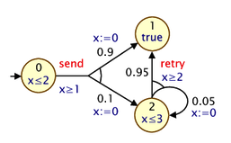
and here is a corresponding PRISM model:
For modelling PTAs in PRISM, there is a new datatype, clock, used for variables that are clocks. Other types of PRISM variables can be defined in the usual way. In the example above, we use just a single integer variable s to represent the locations of the PTAs.
In a PTA, transitions can include a guard, which constrains when it can occur based on the current value of clocks, and resets, which specify that a clock's values should be set to a new (integer) value. These are both specified in PRISM commands in the usual way: see, for example, the inclusion of x>=1 in the guard for the send-labelled command and the updates of the form (x'=0) which reset the clock x to 0.
The other new addition is an invariant construct, which is used to specify an expression describing the clock invariants for each PRISM module. These impose restrictions on the allowable values of clock variables, depending on the values of the other non-clock variables. The invariant construct should appear between the variable declarations and the commands of the module. Often, clock invariants are described separately for each PTA location; hence, the invariant will often take the form of a conjunction of implications, as in the example model above, but more general expressions are also permitted. In the example, the clock x must satisfy x<=2 or x<=3 when local variables s is 0 or 2, respectively. If s is 1, there is no restriction (since the invariant is effectively true in this case).
Expressions that include reference to clocks, whether in guards or invariants, must satisfy certain conditions to facilitate model checking. In particular, references to clocks must appear as conjunctions of simple clock constraints, i.e. conjunctions of expressions of the form x~c or x~y where x and y are clocks, c is an integer-valued expression and ~ is one of <, <=, >=, >, =).
There are also some additional restrictions imposed on PTA models that are dependent on which of the PTA model checking engines is in use.
For the stochastic games and backwards reachability engines:
init...endinit construct is not permitted).
For the digital clocks engine:
x<=5 is allowed, but x<5 is not.
x<=y.
Finally, PRISM makes several assumptions about PTAs, regardless of the engine used.
PRISM supports analysis of partially observable probabilistic models,
most notably partially observable Markov decision processes (POMDPs),
but also partially observable probabilistic timed automata (POPTAs).
POMDPs are a variant of MDPs in which the strategy/policy
which resolves nondeterministic choices in the model is unable to
see the precise state of the model, but instead just observations of it.
For background material on POMDPs and POPTAs, see for example [NPZ17].
You can also find several example models included in the PRISM distribution.
Look in the prism-examples/pomdps and prism-examples/poptas directories.
PRISM currently supports state-based observations: this means that, upon entering a new POMDP state, the observation is determined by that state. In the same way that a model state comprises the values or one or more variables, an observation comprises one or more observables. There are several way to define these observables. The simplest is to specify a subset of the model's variables that are designated as being observable. The rest are unobservable.
For example, in a POMDP with 3 variables, s, l and h, the following:
specifies that s and l are observable and h is not.
Alternatively, observables can be specified as arbitrary expressions over variables.
For example, assuming the same variables s, l and h, this specification:
defines 2 observables. The first is, as above, the variable s.
The second, named "pos", determines if variable l is positive.
Other than this, the values of l and h are unobservable.
The named observables can then be used in properties
in the same way that labels can.
The above two styles of definition can also be mixed to specify a combined set of observables.
POPTAs (partially observable PTAs) combine the features of both PTAs and POMDPs. They are are currently analysed using the digital clocks engine, so inherit the restrictions for that engine. Furthermore, for a POPTA, all clock variables must be observable.
PRISM has support for uncertain models, in which there is epistemic uncertainty regarding some quantitative aspects of the probabilistic models being verified. In particular, it currently supports interval MDPs (IMDPs) and interval DTMCs (IDTMCs), which are MDPs or DTMCs in which transition probabilities can be specified as intervals, indicating that the exact probability is not precisely known. This can be useful, for example, when the transition probabilities have been estimated from data.
Currently, this is achieved by simply replacing the probabilities attached to updates in commands with intervals, e.g.:
As usual, the probability thresholds can be expressions involving state variables or constants, for example:
When two commands in different modules synchronise and specify the probabilities for updates to variables as intervals, these are considered to be independent, i.e., the probability of each combined transition is taken to be the product of the two component intervals.
See the property specification section for details of how these models are analysed.
To make the concept of synchronisation described above more powerful,
PRISM allows you to define precisely the way in which the set of modules are composed in parallel.
This is specified using the system ... endsystem construct,
placed at the end of the model description, which should contain a process-algebraic expression.
This expression should feature each module exactly once, and can use the following (CSP-based) operators:
M1 || M2 : alphabetised parallel composition of modules M1 and M2 (synchronising on only actions appearing in both M1 and M2)
M1 ||| M2 : asynchronous parallel composition of M1 and M2 (fully interleaved, no synchronisation)
M1 |[a,b,...]| M2 : restricted parallel composition of modules M1 and M2 (synchronising only on actions from the set {a, b,...})
M / {a,b,...} : hiding of actions {a, b, ...} in module M
M {a<-b,c<-d,...} : renaming of actions a to b, c to d, etc. in module M.
The first two types of parallel composition (|| and |||) are associative and can be applied to more than two modules at once.
When evaluating the expression, the hiding and renaming operators bind more tightly than the three parallel composition operators.
No other rules of precedence are defined and parentheses should be used to specify the order in which modules are composed.
Some examples of expressions which could be included in the system ... endsystem construct are as follows:
(station1 ||| station2 ||| station3) |[serve]| server
((P1 |[a]| P2) / {a}) || Q
((P1 |[a]| P2) {a<-b}) |[b]| Q
When no parallel composition is specified by the user,
PRISM implicitly assumes an expression of the form M1 || M2 || ... containing all of the modules in the model.
For a more formal definition of the process algebra operators described above, check the semantics of the PRISM language, available from the "Documentation" section of the PRISM web site.
PRISM is also able to import model descriptions written in (a subset of) the stochastic process algebra PEPA [Hil96].
Files containing model descriptions written in the PRISM language
can contain any amount of white space (spaces, tabs, new lines, etc.),
all of which is ignored when the file is parsed by the tool.
Comments can also be used included in files in the style of the C programming language,
by preceding them with the characters //.
This is illustrated by the PRISM language examples from earlier in this section.
We recommend that the .prism extension is used for PRISM model files.
Historically (when the tool supported fewer types of model),
different extensions were often used for each model type:
.nm for MDPs or PTAs, .pm for DTMCs and .sm for CTMCs.


 Site hosted at the Department of Computer Science, University of Oxford