View - Edit - Print - Search

Running PRISM

Starting PRISM

There are two versions of PRISM, one based on a graphical user interface (GUI), the other based on a command line interface. Both use the same underlying model checker. The latter is useful for running large batches of jobs, leaving long-running model checking tasks in the background, or simply for running the tool quickly and easily once you are familiar with its operation.

Details how how to run PRISM can be found in the installation instructions. In short, to run the PRISM GUI:

• (on Windows) click the short-cut (to xprism.bat) installed on the Desktop/Start Menu
• (on other OSs) run the xprism script in the bin directory

You can also optionally specify a model file and a properties file to load upon starting the GUI, e.g.:

To use the command-line version of PRISM, run the prism script, also in the bin directory, e.g.:

The -dir switch can be used to specify a directory for input (and output) files. So the following are equivalent:

The remainder of this section of the manual describes the main types of functionality offered by PRISM. For a more introductory guide to using the tool, try the tutorial on the PRISM web site. Some screenshots of the GUI version of PRISM are shown below.

The PRISM GUI (editing a model)

The PRISM GUI (model checking)

Loading And Building a Model

Typically, when using PRISM, the first step is to load a model that has been specified in the PRISM modelling language. If using the GUI, select menu option "Model | Open Model" and choose a file. There are a selection of sample PRISM model files in the prism-examples directory of the distribution. A few very small models are contained in the subdirectory simple; the rest are in subdirectories grouped by model type.

The model will then be displayed in the editor in the "Model" tab of the GUI window. The file is parsed upon loading. If there are no errors, information about the modules, variables, and other components of the model is displayed in the panel to the left and a green tick will be visible. If there are errors in the file, a red cross will appear instead and the errors will be highlighted in the model editor. To view details of the error, position the mouse pointer over the source of the error (or over the red cross). Alternatively, select menu option "Model | Parse Model" and the error mIessage will be displayed in a message box. Model descriptions can, of course, also be typed from scratch into the GUI's editor.

Building the model

In order to perform model checking, PRISM will (in most cases) need to construct the corresponding probabilistic model, i.e. convert the PRISM model description to, for example, an MDP, DTMC, etc. During this process, PRISM computes the set of states in the model which are reachable from the initial states and the transition matrix which represents the model.

Model construction is done automatically when you perform model checking. However, you may always want to explicitly ask PRISM to build the model in order to test for errors or to see how large the model is. From the GUI, you can do this by by selecting "Model | Build Model". If there are no errors during model construction, the number of states and transitions in the model will be displayed in the bottom left corner of the window.

From the command-line, simply type:

where model.nm is the name of the file containing the model description.

For some types of models, notably PTAs, models are not constructed in this way (because the models are infinite-state). In these cases, analysis of the model is not performed until model checking is performed.

Deadlocks

You should be aware of the possibility of deadlock states (or deadlocks) in the model, i.e. states which are reachable but from which there are no outgoing transitions. PRISM will automatically search your model for deadlocks and, by default, "fix" them by adding self-loops in these states. Since deadlocks are sometimes caused by modelling errors, PRISM will display a warning message in the log when deadlocks are fixed in this way.

You can control whether deadlocks are automatically fixed in this way using the "Automatically fix deadlocks" option (or with command-line switches -nofixdl and -fixdl). When fixing is disabled, PRISM will report and error when the model contains deadlocks (this used to be the default behaviour in older versions of PRISM).

If you have unwanted or unexpected deadlocks in your model, there are several ways you can detect then. Firstly, by disabling deadlock fixing (as described above), PRISM will display a list of deadlock states in the log. Alternatively, you can model check the filter property filter(print, "deadlock"), which has the safe effect.

To find out how deadlocks occur, i.e. which paths through the model lead to a deadlock state, there are several possibilities. Firstly, you can model check the CTL property E[F "deadlock"]. When checked from the GUI, this will provide you with the option of display a path to a deadlock in the simulator. From the command-line, for example with:

a path to a deadlock will be displayed in the log.

Finally, in the eventuality that the model is too large to be model checked, you can still use the simulator to search for deadlocks. This can be done either by manually generating random paths using the simulator in the GUI or, from the command-line, e.g. by running:

Debugging Models With The Simulator

PRISM includes a simulator, a tool which can be used to generate sample paths (executions) through a PRISM model. From the GUI, the simulator allows you to explore a model by interactively generating such paths. This is particularly useful for debugging models during development and for running sanity checks on completed models. Paths can also be generated from the command-line.

Generating a path in the GUI

Once you have loaded a model into the PRISM GUI (note that it is not necessary to build the model), select the "Simulator" tab at the bottom of the main window. You can now start a new path by double-clicking in the bottom half of the window (or right-clicking and selecting "New path"). If there are undefined constants in the model (or in any currently loaded properties files) you will be prompted to give values for these. You can also specify the state from which you wish to generate a path. By default, this is the initial state of the model.

The main portion of the user interface (the bottom part) displays a path through the currently loaded model. Initially, this will comprise just a single state. The table above shows the list of available transitions from this state. Double-click one of these to extend the path with this transition. The process can be repeated to extend the path in an interactive fashion. Clicking on any state in the current path shows the transition which was taken at this stage. Click on the final state in the path to continue extending the path. Alternatively, clicking the "Simulate" button will select a transition randomly (according to the probabilities/rates of the available transitions). By changing the number in the box below this button, you can easily generate random paths of a given length with a single click. There are also options (in the accompanying drop-down menu) to allow generation of paths up until a particular length or, for CTMCs, in terms of the time taken.

The figure shows the simulator in action.

The PRISM GUI: exploring a model using the simulator

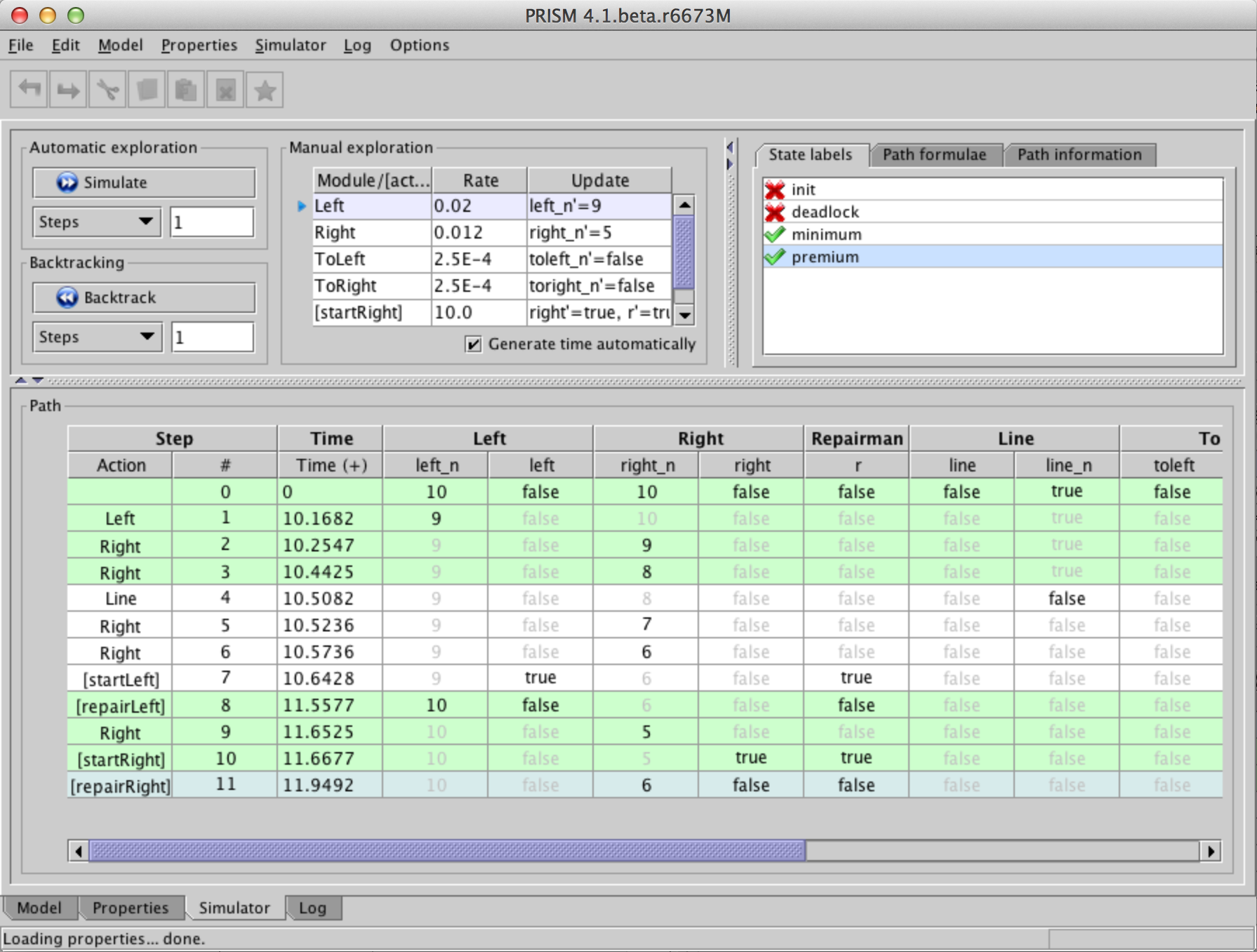
It is also possible to:

• backtrack to an earlier point in a path
• remove all of the states before some point in a path
• restart a path from its first state
• export a path to a text file

Notice that the table containing the path displays not just the value of each variable in each state but also the time spent in that state and any rewards accumulated there. You can configure exactly which columns appear by right-clicking on the path and selecting "Configure view". For rewards (and for CTMC models, for the time-values), you can can opt to display the reward/time for each individual state and/or the cumulative total up until each point in the path.

At the top-right of the interface, any labels contained in the currently loaded model/properties file are displayed, along with their value in the currently selected state of the path. In addition, the built-in labels "init" and "deadlock" are also included. Selecting a label from the list highlights all states in the current path which satisfy it.

The other tabs in this panel allow the value of path operators (taken from properties in the current file) to be viewed for the current path, as well as various other statistics.

Another very useful feature for some models is to use the "Plot new path" option from the simulator, which generates a plot of some/all of the variable/reward values for a particular randomly generated path through the model.

Path generation from the command-line

It is also possible to generate random paths through a model using the command-line version of PRISM. This is achieved using the -simpath switch, which requires two arguments, the first describing the path to be generated and the second specifying the file to which the path should be output (as usual, specifying stdout sends output to the terminal). The following examples illustrate the various ways of generating paths in this way:

These generate a path of 10 steps, a path of at least 7.5 time units and a path ending in deadlock, respectively.

Here's an example of the output:

This shows the sequence of states in the path, i.e. the values of the variables in each state. In the example above, there are 4 variables: s, a, s1 and s2. The first three columns show the type of transition taken to reach that state, its index within the path (starting from 0) and the time at which it was entered. The latter is only shown for continuous time models. The type of the transition is written as [act] if action label act was taken, and as module1 if the module named module1 takes an unlabelled transition).

Further options can also be appended to the first parameter. For example, option probs=true also displays the probability/rate associated with each transition. For example:

In this example, the rate is 200.0 for all transitions. To show the state/transition rewards for each step, use option rewards=true.

If you are only interested in values of certain variables of your model, use the vars=(...) option. For example:

Note the use of single quotes around the path description argument to prevent the shell from misinterpreting special characters such as "(".

Notice also that the above only displays states in which the values of some variable of interest changes. This is achieved with the option changes=true, which is automatically enabled when you use vars=(...). If you want to see all steps of the path, add the option changes=false.

An alternative way of viewing paths is to only display paths at certain fixed points in time. This is achieved with the snapshot=x option, where x is the time step. For example:

You can also use the sep=... option to specify the column separator. Possible values are space (the default), tab and comma. For example:

When generating paths to a deadlock state, additional repeat=... option is available which will construct multiple paths until a deadlock is found. For example:

By default, the simulator detects deterministic loops in paths (e.g. if a path reaches a state from which there is a just a single self-loop leaving that state) and stops generating the path any further. You can disable this behaviour with the loopcheck=false option. For example:

One final note: the -simpath switch only generates paths up to the maximum path length setting of the simulator (the default is 10,000). If you want to generate longer paths, either change the default setting or override it temporarily from the command-line using the -simpathlen switch. You might also use the latter to decrease the setting, e.g. to look for a path leading to a deadlock state, but only within 100 steps:

Exporting The Model

If required, once the model has been constructed, it can be exported, either for manual examination or for use in another tool. The following can all be exported:

• the set of reachable states;
• the transition matrix;
• the state rewards vector(s);
• the transition rewards matrix (or matrices).
• labels (in the model or properties) and the states that satisfy them

Note that the last of these also provides a way to export information about initial states and deadlock states (via the built-in labels "init" and "deadlock").

From the GUI, use the "Model | Export" menu to export the data to a file or, for small models, use the "Model | View" menu to print the details directly to the log. For the case of labels, if you want to export labels from the properties file too, use the "Properties | Export labels" option, rather than the "Model | Export" one.

From the command-line version of PRISM, use the following switches:

• -exportstates <file>
• -exporttrans <file>
• -exportstaterewards <file>
• -exporttransrewards <file>
• -exportlabels <file>

or, as explained below, use the more convenient switch:

• -exportmodel <files[:options]>

Replace <file> with stdout in any of the above to print the information to the terminal.

The export command-line switches can be used in combination. For example:

exports both the state space and transition matrix. You can export both state and transition rewards using the -exportrewards switch. The following are equivalent:

When there are multiple reward structures, a separate file is created for each one and a (1-indexed) suffix is added to distinguish them. A header in each file (see the "Explicit Model Files" appendix) also shows the name of the reward structure. These headers can be omitted using the switch -noexportheaders (or via the option "Include headers in model exports" in the GUI).

You can also easily perform multiple exports simultaneously using the -exportmodel switch, which specifies multiple files using a list of extensions. The file extensions then dictate what is exported. For example:

exports the transition matrix and states list to out.tra and out.sta, respectively. If you omit the file basename (out in this case), then the basename of the model file (poll2 in this case) is used. For example:

exports the transition matrix and states list to poll2.tra and poll2.sta.

Possible file extensions are: .sta (reachable states), .tra (transition matrix), .srew (state rewards), .trew (transition rewards), .lab (labels). You can use the shorthand .all to export everything, and .rew to export both state and transition rewards. For example:

creates multiple files of the form out.* or poll2.*, respectively.

As mentioned above, you can always use stdout instead of a filename. For example:

is a quick way to print all details (of a small model) to the terminal.

Although it is not exported when using .all, the -exportmodel switch can also be used to export the transition matrix in Dot format which allows easy graphical visualisation of the model:

Export options

When exporting model details in this way, the precision of numerical values (e.g., for probabilities or rewards) can be configured. From the command line, use the switch -exportmodelprecision <x> to show values to <x> significant digits. The same setting is available for exports from the GUI via option "Precision of model export".

Finally, the -exportmodel switch can be passed various options. The general form is -exportmodel files:options where options is a comma-separated list of options taken from the following list:

• mrmc - export data in MRMC format
• matlab - export data in Matlab format
• rows - export matrices with one row/distribution on each line
• ordered - output states indices in ascending order [default]
• unordered - don't output states indices in ascending order
• proplabels - also export labels from the properties file

An example is:

By default, when labels are exported, this only includes the labels from the model. The proplabels option listed above (which applies to both -exportmodel and -exportlabels) indicates that labels from any properties file are exported too. To export just those labels, use switch -exportproplabels <file>.

File formats

By default, model data is exported (or displayed) in plain text format. The precise details of the formats used can be found in the "Explicit Model Files" appendix. As mentioned above, by convention, we use file extensions .sta (for states files), .tra (for transitions files), .srew and .trew (for state/transition rewards files) and .lab (for labels).

Alternatively, it is possible to export this information as Matlab code (a .m file) or in a format suitable for import into the MRMC tool. Select the appropriate menu item when using the GUI, or add the command-line switches:

• -exportmatlab
• -exportmrmc

or, as described earlier, pass options to the -exportmodel switch.

There is no specific MRMC format for labels, so these are exported as plain text in this case.

There is some additional export functionality available only from the command-line.

Firstly, when outputting matrices for DTMCs or CTMCs, it is possible to request that PRISM does not sort the rows of the matrix, as is normally the case. This is achieved with the switch:

• -exportunordered

The reason for this is that in this case PRISM does not need to construct an explicit version of the model in memory and the process can thus be performed with reduced memory consumption.

Secondly, there is a switch:

• -exportrows

which provides an alternative output format for transition matrices where the elements of each row of the matrix (i.e. the transitions from a state/choice) are grouped on the same line. This can be particularly helpful for viewing the matrix for MDPs. The file format is shown here.

Graphical model export

The transition matrix of the model can also be exported in Dot format, which allows easy graphical visualisation of the graph structure of the model. You can optionally request that state descriptions are added to each state of graph; if not, states are labelled with integer indices that can be cross-referenced with the list of reachable states.

Use the menu entries under "Model | Export | Transition matrix" from the GUI or command-line switches:

• -exporttransdot <file>
• -exporttransdotstates <file>

As mentioned above, for the latter, the following is equivalent (and easier to remember):

Exporting (B)SCCs and end components

It is also possible to export the set of (bottom) strongly connected components (SCCs or BSCCs) for a model. This can only be done from the command-line currently. Use, for example:

For an MDP, you can also export the set of maximal end components (MECs):

Model Checking

Typically, once a model has been constructed, it is analysed through model checking. Properties are specified as described in the "Property Specification" section, and are usually kept in files with extensions .props, .pctl or .csl. There are properties files accompanying most of the sample PRISM models in the prism-examples directory.

GUI

To load a file containing properties into the GUI, select menu option "Properties | Open properties list". The file can only be loaded if there are no errors, otherwise an error is displayed. Note that it may be necessary to have loaded the corresponding model first, since the properties will probably make reference to variables (and perhaps constants) declared in the model file. Once loaded, the properties contained in the file are displayed in a list in the "Properties" tab of the GUI. Constants and labels are displayed in separate lists below. You can modify or create new properties, constants and labels from the GUI, by right-clicking on the appropriate list and selecting from the pop-up menu which appears. Properties with errors are shaded red and marked with a warning sign. Positioning the mouse pointer over the property displays the corresponding error message.

The pop-up menu for the properties list also contains a "Verify" option, which allows you instruct PRISM to model check the currently selected properties (hold down Ctrl/Cmd to select more than one property simultaneously). All properties can be model checked at once by selecting "Verify all". PRISM verifies each property individually. Upon completion, the icon next to the property changes according to the result of model checking. For Boolean-valued properties, a result of true or false is indicated by a green tick or red cross, respectively. For properties which have a numerical result (e.g. P=? [ ...]), position the mouse pointer over the property to view the result. In addition, this and further information about model checking is displayed in the log in the "Log" tab.

Command-line

From the command-line, model checking is achieved by passing both a model file and a properties file as arguments, e.g.:

The results of model checking are sent to the display and are as described above for the GUI version. By default, all properties in the file are checked. To model check only a single property, use the -prop switch. For example, to check only the fourth property in the file:

or to check only the property with name "safe" in the file:

You can also provide a comma-separated list of multiple properties to check, using neither numerical indices or property names:

Alternatively, the contents of a properties file can be specified directly from the command-line, using the -pf switch:

The switches -pctl and -csl are aliases for -pf.

Note the use of single quotes ('...') to avoid characters such as ( and > being interpreted by the command-line shell. Single quotes are preferable to double quotes since PRISM properties often include double quotes, e.g. for references to labels or properties.

Approximate Model Checking

The discrete-event simulator built into PRISM (see the section "Debugging Models With The Simulator") can also be used to generate approximate results for PRISM properties, a technique often called statistical model checking. Essentially, this is achieved by sampling: generating a large number of random paths through the model, evaluating the result of the given properties on each run, and using this information to generate an approximately correct result. This approach is particularly useful on very large models when normal model checking is infeasible. This is because discrete-event simulation is performed using the PRISM language model description, without explicitly constructing the corresponding probabilistic model.

Currently, statistical model checking can only be applied to P or R operators and does not support LTL-style path properties or filters. There are also a few restrictions on the modelling language features that can be used; see below for details.

To use this functionality, load a model and some properties into PRISM, as described in the previous sections. To generate an approximate value for one or more properties, select them in the list, right-click and select "Simulate" (as opposed to "Verify"). As usual, it is first necessary to provide values for any undefined constants. Subsequently, a dialog appears. Here, the state from which approximate values are to be computed (i.e. from which the paths will be generated) can be selected. By default, this is the initial state of the model. The other settings in the dialog concern the methods used for simulation.

PRISM supports four different methods for performing statistical model checking:

• CI (Confidence Interval)
• ACI (Asymptotic Confidence Interval)
• APMC (Approximate Probabilistic Model Checking)
• SPRT (Sequential Probability Ratio Test)

The first three of these are intended primarily for "quantitative" properties (e.g. of the form P=?[...]), but can also be used for "bounded" properties (e.g. of the form P<p[...]). The SPRT method is only applicable to "bounded" properties.

Each method has several parameters that control its execution, i.e. the number of samples that are generated and the accuracy of the computed approximation. In most cases, these parameters are inter-related so one of them must be left unspecified and its value computed automatically based on the others. In some cases, this is done before simulation; in others, it must be done afterwards.

Below, we describe each method in more detail. For simplicity, we describe the case of checking a P operator. Details for the case of an R operator can be found in [Nim10].

CI (Confidence Interval) Method

The CI method gives a confidence interval for the approximate value generated for a P=? property, based on a given confidence level and the number of samples generated. The parameters of the method are:

• "Width" (w)
• "Confidence" (alpha)
• "Number of samples" (N)

Let X denote the true result of the query P=?[...] and Y the approximation generated. The confidence interval is [Y-w,Y+w], i.e. w gives the half-width of the interval. The confidence level, which is usually stated as a percentage, is 100(1-alpha)%. This means that the actual value X should fall into the confidence interval [Y-w,Y+w] 100(1-alpha)% of the time.

To determine, for example, the width w for given alpha and N, we use w = q * sqrt(v / N) where q is a quantile, for probability 1-alpha/2, from the Student's t-distribution with N-1 degrees of freedom and v is (an estimation of) the variance for X. Similarly, we can determine the required number of iterations, from w and alpha, as N = (v * q²)/w², where q and v are as before.

For a bounded property P~p[...], the (Boolean) result is determined according to the generated approximation for the probability. This is not the case, however, if the threshold p falls within the confidence interval [Y-w,Y+w], in which case no value is returned.

ACI (Asymptotic Confidence Interval) Method

The ACI method works in exactly same fashion as the CI method, except that it uses the Normal distribution to approximate the Student's t-distribution when determining the confidence interval. This is appropriate when the number of samples is large (because we can get a reliable estimation of the variance from the samples) but may be less accurate for small numbers of samples.

APMC (Approximate Probabilistic Model Checking) Method

The APMC method, based on [HLMP04], offers a probabilistic guarantee on the accuracy of the approximate value generated for a P=? property, based on the Chernoff-Hoeffding bound. The parameters of the method are:

• "Approximation" (epsilon)
• "Confidence" (delta)
• "Number of samples" (N)

Letting X denote the true result of the query P=?[...] and Y the approximation generated, we have:

• Prob(|Y-X| > epsilon) < delta

where the parameters are related as follows: N = ln(2/delta) / 2epsilon². This imposes certain restrictions on the parameters, namely that N(epsilon²) ≥ ln(2)/2.

In similar fashion to the CI/ACI methods, the APMC method can be also be used for bounded properties such as P~p[...], as long as the threshold p falls outside the interval [Y-epsilon,Y+epsilon].

SPRT (Sequential Probability Ratio Test) Method

The SPRT method is specifically for bounded properties, such as P~p[...] and is based on acceptance sampling techniques [YS02]. It uses Wald's sequential probability ratio test (SPRT), which generates a succession of samples, deciding on-the-fly when an answer can be given with a sufficiently high confidence.

The parameters of the method are:

• "Indifference" (delta)
• "Type I/II error" (alpha/beta)

Consider a property of the form P≥p[...]. The parameter delta is used as the half-width of an indifference region [p-delta,p+delta]. PRISM will attempt to determine whether either the hypothesis P≥(p+delta)[...] or P≤(p-delta)[...] is true, based on which it will return either true or false, respectively. The parameters alpha and beta represent the probability of the occurrence of a type I error (wrongly accepting the first hypothesis) and a type II error (wrongly accepting the second hypothesis), respectively. For simplicity, PRISM assigns the same value to both alpha and beta.

Maximum Path Length

Another setting that can be configured from the "Simulation Parameters" dialog is the maximum length of paths generated by PRISM during statistical model checking. In order to perform statistical model checking, PRISM needs to evaluate the property being checked along every generated path. For example, when checking P=? [ F<=10 "end" ], PRISM must check whether F<=10 "end" is true for each path. On this example (assuming a discrete-time model), this can always be done within the first 10 steps. For a property such as P=? [ F "end" ], however, there may be paths along which no finite fragment can show F "end" to be true or false. So, PRISM imposes a maximum path length to avoid the need to generate excessively long (or infinite) paths. The default maximum length is 10,000 steps. If, for a given property, statistical model checking results in one or more paths on which the property can be evaluated, an error is reported.

Command-line Statistical Model Checking

Statistical model checking can also be enabled from the command-line version of PRISM, by including the -sim switch. The default methods used are CI (Confidence Interval) for "quantitative" properties and SPRT (Sequential Probability Ratio Test) for "bounded" properties. To select a particular method, use switch -simmethod <method> where <method> is one of ci, aci, apmc and sprt. For example:

PRISM has default values for the various simulation method parameters, but these can also be specified using the switches -simsamples, -simconf, -simwidth and -simapprox. The exact meaning of these switches for each simulation method is given in the table below.

The maximum length of simulation paths is set with switch -simpathlen.

Limitations

Currently, the simulator does not support every part of the PRISM modelling languages. For example, it does not handle models with multiple initial states or with system...endsystem definitions.

It is also worth pointing out that statistical model checking techniques are not well suited to models that exhibit nondeterminism, such as MDPs. This because the techniques rely on generation of random paths, which are not well defined for a MDP. PRISM does allow statistical model checking to be performed on an MDP, but does so by simply resolving nondeterministic choices in a (uniformly) random fashion (and displaying a warning message). Currently PTAs are not supported by the simulator.

Computing Steady-state And Transient Probabilities

If the model is a CTMC or DTMC, it is possible to compute corresponding vectors of steady-state or transient probabilities directly (rather than indirectly by analysing a property which requires their computation). From the GUI, select an option from the "Model | Compute" menu. For transient probabilities, you will be asked to supply the time value for which you wish to compute probabilities. From the command-line, add the -steadystate (or -ss) switch:

for steady-state probabilities or the -transient (or -tr) switch:

for transient probabilities, again specifying a time value in the latter case. The probabilities are computed for all states of the model and displayed, either on the screen (from the command-line) or in the log (from the GUI).

To instead export the vector of computed probabilities to a file, use the "Model | Compute/export" option from the GUI, or the -exportsteadystate (or -exportss) and -exporttransient (or -exporttr) switches from the command-line:

From the command-line, you can request that the probability vectors exported are in Matlab format by adding the -exportmatlab switch.

Initial probability distributions

By default, for both steady-state and transient probability computation, PRISM assumes that the initial probability distribution of the model is an equiprobable choice over the set of initial states. You can override this and provide a specific initial distribution. This is done using the -importinitdist switch. The format for this imported distribution is identical to the ones exported by PRISM, i.e. simply a list of probabilities for all states separated by new lines. For example, this:

is (essentially) equivalent to this:

Ranges of time values

Finally, you can compute transient probabilities for a range of time values, e.g.:

which computes transient probabilities for the time points 0.1, 0.11, 0.12, .., 0.2. In this case, the computation is done incrementally, with probabilities for each time point being computed from the previous point for efficiency.

Experiments

PRISM supports experiments, which is a way of automating multiple instances of model checking. This is done by leaving one or more constants undefined, e.g.:

This can be done for constants in the model file, the properties file, or both. Before any verification can be performed, values must be provided for any such constants. In the GUI, a dialog appears in which the user is required to enter values. From the command line, the -const switch must be used, e.g.:

To run an experiment, provide a range of values for one or more of the constants. Model checking will be performed for all combinations of the constant values provided. For example:

where N=4:6 means that values of 4,5 and 6 are used for N, and T=60:10:100 means that values of 60, 70, 80, 90 and 100 (i.e. steps of 10) are used for T.

For convenience, constant specifications can be split across separate instances of the -const switch, if desired. You can also specify double-valued constants as fractions rather than decimals. For example:

From the GUI, the same thing can be achieved by selecting a single property, right clicking on it and selecting "New experiment" (or alternatively using the popup menu in the "Experiments" panel). Values or ranges for each undefined constant can then be supplied in the resulting dialog. Details of the new experiment and its progress are shown in the panel. To stop the experiment before it has completed, click the red "Stop" button and it will halt after finishing the current iteration of model checking. Once the experiment has finished, right clicking on the experiment produces a pop-up menu, from which you can view the results of the experiment or export them to a file.

For experiments based on properties which return numerical results, you can also use the GUI to plot graphs of the results. This can be done either before the experiment starts, by selecting the "Create graph" tick-box in the dialog used to create the experiment (in fact this box is ticked by default), or after the experiment's completion, by choosing "Plot results" from the pop-up menu on the experiment. A dialog appears, where you can choose which constant (if there are more than one) to use for the x-axis of the graph, and for which values of any other constants the results should be plotted. The graph will appear in the panel below the list of experiments. Right clicking on a graph and selecting "Graph options" brings up a dialog from which many properties of the graph can be configured. From the pop-up menu of a graph, you can also choose to print the graph (to a printer or Postscript file) or export it in a variety of formats: as an image (PNG or JPEG), as an encapsulated Postscript file (EPS), in an XML-based format (for reloading back into PRISM), or as code which can be used to generate the graph in Matlab.

Approximate computation of quantitive results obtained with the simulator can also be used on experiments. In the GUI, select the "Use Simulation" option when defining the parameters for the experiment. From the command-line, just add the -sim switch as usual.

Exporting results

You can export all the results from an experiment to a file or to the screen. From the command-line, use the -exportresults switch, for example:

to send to output file res.txt, or:

to send the results straight to the screen. From the GUI, right click on the experiment and select "Export results".

The default behaviour is to export a list of results in text form, using tabs to separate items. The above examples produce:

You can change the format in which the results are exported by appending one or more comma-separated options to the end of the -exportresults switch, for example to export in CSV (comma-separated values) format:

or in DataFrame format:

You can also add the matrix option, to export the results as one or more 2D matrices, rather than a list. This is particularly useful if you want to create a surface plot from results that vary over two constants.

The matrix option is also available in normal (non-CSV) mode.

You can also export results in the form of comments, used by PRISM's regression testing functionality:

From the GUI, it is also possible to import previously exported results (in DataFrame format).

A related option is the -exportvector <file> switch, useful in general contexts, not for experiments. This exports the results for all states of the model (typically, the log just displays the result for the initial state, unless a filter has been used) to the the file file.

Strategies

Properties to be model checked on MDPs (and their variants, such as POMDPs or IMDPs) usually quantify over strategies (or policies) of the model, i.e., over the different possible ways that nondeterminism can be resolved in the model. For example, this property:

determines the maximum probability, over all strategies, of reaching a state satisfying the label "goal". When checking such properties, you can also ask PRISM to generate a corresponding (optimal) strategy, which yields this maximum probability when followed. The strategy can then be viewed, exported or simulated.

Note: For consistency across models, PRISM now uses the terminology strategy (rather than alternatives such as policy). In older versions of the tool, these were referred to as adversaries. Currently, the newer (and more extensive) strategy generation functionality is implemented just for the "explicit" model checking engine, which is used automatically if strategy generation is requested. The old adversary generation functionality (see below) still exists for the "sparse" engine, but will be updated in the future.

Generating strategies. Optimal strategies can be generated either from the command-line or the graphical user interface (GUI). For the former, use the -exportstrat switch. Simple examples are:

From the GUI, you can trigger strategy generation by ticking the "Generate strategy" box either on the popup menu that appears when you right-click a property, or from the "Strategies" menu at the top. As long as it is supported, a strategy will be then generated once "Verify" is clicked.

From the same menu(s), you can then

• export the strategy to a file
• view the strategy by printing it in the log
• explore the strategy in the simulator

Strategy export types. Strategies can be viewed or exported in several different formats:

(i) Action list. This is a list of the action taken in each state of the model, e.g.:

where states, by default, are shown as a tuple of variable values.

(ii) Induced model. This is a representation of the model that is induced when the strategy is applied. There are two "modes" for this export: restrict, which shows the original model but with a restricted set of choices (e.g., an MDP with just one choice in each state); and reduce, which removes the nondeterminism resolved by the strategy (e.g., an MDP becomes a DTMC). The latter can be useful to re-import the model back into PRISM and analyse the induced model; the former is sometimes easier for visualising the strategy's choices. In each case, the transitions of the induced model are presented as a .tra file (as for normal model export), e.g.:

(iii) Dot file. This is, like the previous format, a view of the model induced by the strategy, but in Dot format, which allows it to be visualised.

Configuring strategy export. As hinted in the command-line examples above, the -exportstrat switch uses the file extension to determine the preferred format: if the strategy is exported to a file with extension .tra or .dot, then it uses an induced model or Dot file, respectively. Otherwise, the default is an action list. You can specify the desired format:

Further options can be added, e.g., to specify whether an induced model is exported in "restrict" or "reduce" mode:

A full list of available options is as follows:

• type (actions, induced or dot): the type of strategy export to use (action list, induced model or Dot file)
• mode (restrict or reduce): when exporting as an induced model or Dot file, whether to "restrict" or "reduce" the model (see above); the default is "restrict"
• reach (true or false): whether to restrict the strategy to states that are reachable when it is applied to the model (this is currently only used for exporting induced models and Dot files, and the default value is false and true, respectively, in these two cases)
• states (true or false): whether to show states, rather than state indices, for actions lists or Dot files; this is true by default
• obs (true or false): for partially observable models, whether to merge observationally equivalent states; this is true by default

Strategy types. PRISM generates several types of strategies. The simplest are memoryless deterministic strategies, which pick a single action in each state, as in the examples above. For some query types (e.g., step-bounded properties, or LTL-based properties), finite-memory strategies are generated, where an additional memory value is used. For these, induced models or Dot files are most useful since they will also show how the memory values are updated as the strategy is executed. Note that, in these cases, the state indices of the strategy will correspond to the product model constructed during model checking, not the original model. The product model can be exported using the -exportprodtrans and -exportprodstates switches.

Adversary generation. As mentioned above, the "sparse" model checking engine still includes older so-called "adversary generation" functionality. This can be used to export the induced model to a file using the -exportadv switch, e.g.:

where the -exportadv and -exportadvmdp export a DTMC and an MDP, respectively, i.e., corresponding to the "reduce" and "restrict" modes described above. From the GUI, change the "Adversary export" option (under the "PRISM" settings) from "None" to "DTMC" or "MDP". You can also change the filename for the export adversary which, by default, is adv.tra as in the example above.

Support For PEPA Models

For CTMCs, PRISM also accepts model descriptions in the stochastic process algebra PEPA [Hil96]. The tool compiles such descriptions into the PRISM language and then constructs the model as normal. The language accepted by the PEPA to PRISM compiler is actually a subset of PEPA. The restrictions applied to the language are firstly that component identifiers can only be bound to sequential components (formed using prefix and choice and references to other sequential components only). Secondly, each local state of a sequential component must be named. For example, we would rewrite:

• P = (a,r).(b,s).P;

as:

• P = (a,r).P';
• P' = (b,s).P;

Finally, active/active synchronisations are not allowed since the PRISM definition of these differs from the PEPA definition. Every PEPA synchronisation must have exactly one active component. Some examples of PEPA model descriptions which can be imported into PRISM can be found in the prism-examples/pepa directory.

From the command-line version of PRISM, add the -importpepa switch and the model will be treated as a PEPA description. From the GUI, select "Model | Open model" and then choose "PEPA models" on the "Files of type" drop-down menu. Alternatively, select "Model | New | PEPA model" and either type a description from scratch or paste in an existing one from elsewhere. Once the PEPA model has been successfully parsed by PRISM, you can view the corresponding PRISM code (as generated by the PEPA-to-PRISM compiler) by selecting menu option "Model | View | Parsed PRISM model".

Support For SBML

PRISM includes a (prototype) tool to translate specifications in SBML (Systems Biology Markup Language) to model descriptions in the PRISM language. SBML is an XML-based format for representing models of biochemical reaction networks. The translator currently works with Level 2 Version 1 of the SBML specification, details of which can be found here.

Since PRISM is a tool for analysing discrete-state systems, the translator is designed for SBML files intended for discrete stochastic simulation. A useful set of such files can be found in the CaliBayes Discrete Stochastic Model Test Suite. There are also many more SBML files available in the BioModels Database.

We first give a simple example of an SBML file and its PRISM translation. We then give some more precise details of the translation process.

Example

An SBML file comprises a set of species and a set of reactions which they undergo. Below is the SBML file for the simple reversible reaction: Na + Cl ↔ Na⁺ + Cl^-, where there are initially 100 Na and Cl atoms and no ions, and the base rates for the forwards and backwards reactions are 100 and 10, respectively.

And here is the resulting PRISM code:

From the latter, we can use PRISM to generate a simple plot of the expected amount of Na and Na+ over time (using both model checking and a single random trace from the simulator):

Expected amount of Na/Na+ at time T

Using the translator

At present, the SBML-to-PRISM translator is included in the PRISM code-base, but not integrated into the application itself.

If you are using a binary (rather than source code) distribution of PRISM, replace classes with lib/prism.jar in the above.

Alternatively (on Linux or Mac OS X), ensure prism is in your path and then save the script below as an executable file called sbml2prism:

Then use:

The following PRISM properties file will also be useful:

This contains a single property which, based on the reward structures in the PRISM model generated by the translator, means "the expected amount of species c at time T". The constant c is an integer index which can range between 1 and N, where N is the number of species in the model. To view the expected amount of each species over time, create an experiment in PRISM which varies c from 1 to N and T over the desired time range.

Details of the translation

The basic structure of the translation process is as follows:

• Each species in the SBML file is represented by a module in the resulting PRISM file. This module, which (where possible) retains the SBML species id as its name, contains a single variable whose value represents the amount of the species present. A corresponding reward structure for computing the expected amount of the species at a given time instant is also created. Species for which the boundaryCondition flag is set to true in the SBML file do not have a corresponding module.
• Each reaction in the SBML file is associated with a unique synchronisation action label. The module for each species which takes part in the reaction will include a synchronous command to represent this. An additional PRISM module called reaction_rates stores the expression representing the rate of each reaction (from the corresponding kineticLaw section in the SBML file). Reaction stoichiometry information is respected but must be provided in the scalar stoichiometry field of a speciesReference element, not in a separate StoichiometryMath element.
• Each parameter in the SBML file, either global to the file or specific to a reaction, becomes a constant in the PRISM file. If a value for this parameter is given, it used. If not, the constant is left as undefined.

As described above, this translation process is designed for discrete systems and so the amount of each species in the model is represented by an integer variable. It is therefore assumed that the initial amount for each species specified in the SBML file is also given as an integer. If this is not the case, then the values will need to be scaled accordingly first.

Furthermore, since PRISM is primarily a model checking (rather than simulation) tool, it is important that the amount of each species also has an upper bound (to ensure a finite state space). When model checking, the efficiency (or even feasibility) of the process is likely to be very sensitive to the upper bound(s) chosen. When using the discrete-event simulation functionality of PRISM, this is not the case and the bounds can can be set much higher. By default the translator uses an upper bound of 100 (which is increased if the initial amount exceeds this). A different value can specified through a second command-line argument as follows:

Alternatively, upper bounds can be modified manually after the translation process.

Finally, The following aspects of SBML files are not currently supported and are ignored during the translation process:

• compartments
• events/triggers

Explicit Model Import

It is also possible to construct models in PRISM through direct specification of their transition matrix. The format in which this information is input to the tool is exactly the same as is currently output (see the section "Exporting The Model" and the appendix "Explicit Model Files"). Presently, this functionality is only supported in the command-line version of the tool, using the -importtrans switch (and more convenient -importmodel; see below). PRISM makes some attempt to discern the model type from the format of the input files, but if this does not work, the model type can be overwritten using the -dtmc, -ctmc and -mdp switches. For example:

Please note that this method of constructing models in PRISM is typically less efficient than using the PRISM language. This is because PRISM is (primarily) a symbolic model checker and the underlying data structures used to represent the model function better when there is high-level structure and regularity to exploit. This situation can be alleviated to a certain extent by importing not just a transition matrix, but also a definition of each state of the model in terms of a set of variables. The format of this information is again identical to PRISM's current output format, using the -exportstates switch. The following example shows how PRISM could be used to build, export and then re-import a model (not a good strategy in general):

You can also import label information using the switch -importlabels, e.g.:

where the labels file (poll2.lab above) is in the format generated by the -exportlabels export option of PRISM.

In particular, since details about the initial state(s) of a model are not preserved in the files output from -exportstates and -exporttrans, but are included in the labels file, -importlabels should also be used to designate a particular initial state for a model. If not, the default is to assume a single initial state, in which all variables take their minimum value (if -importstates is not used, the model has a a single zero-indexed variable x, and the initial state is x=0).

Lastly, state (but currently not transition) rewards can also be imported, using the -importstaterewards switch, e.g.:

You can import multiple reward structures using multiple instances of the -importstaterewards switch. If present in the rewards files (see the appendix "Explicit Model Files"), the names of the reward structures are read too.

In a similar style to PRISM's -exportmodel switch, you can import several several files for a model using a single -importmodel switch. For example, this is equivalent to the command given above:

The contents of each file is determined by its extension: Possible file extensions are: .sta (reachable states), .tra (transition matrix), .lab (labels), .srew (state rewards).

Use the extension .all to import from all of these files:

In this case, you can omit the -importmodel switch and just specify the .all-ended filename, e.g.: