
(Hermanns, Meyer-Kayser & Siegle)
This case study is based on a simple tandem queueing network, taken from [HMKS99]. The model is represented as a CTMC which consists of a M/Cox2/1-queue sequentially composed with a M/M/1-queue. We use c to denote the capacity of the queues. The PRISM source code is given below.
// tandem queueing network [HKMKS99]
// gxn/dxp 25/01/00

ctmc

const int c; // queue capacity

const double lambda = 4*c;
const double mu1a = 0.1*2;
const double mu1b = 0.9*2;
const double mu2 = 2;
const double kappa = 4;

module serverC

	sc : [0..c];
	ph : [1..2];

	[] (sc<c) -> lambda: (sc'=sc+1);
	[route] (sc>0) & (ph=1) -> mu1b: (sc'=sc-1);
	[] (sc>0) & (ph=1) -> mu1a: (ph'=2);
	[route] (sc>0) & (ph=2) -> mu2: (ph'=1) & (sc'=sc-1);

endmodule

module serverM

	sm : [0..c];

	[route]	(sm<c) -> 1: (sm'=sm+1);
	[] (sm>0) -> kappa: (sm'=sm-1);

endmodule

// reward - number of customers in network
rewards "customers"
	true : sc + sm;
endrewards
The table below shows statistics for each model we have built. The first section gives information about the CTMC representing the model: the number of states and the number of non-zeros (transitions). The second part refers to the MTBDD which represents this CTMC: the total number of nodes, the number of leaves (terminal nodes), and the amount of memory needed to store it. The last column gives the amount of memory a sparse matrix would need to represent the same CTMC.
| c: | Model: | MTBDD: | Sparse: | ||||||
| States: | NNZ: | Nodes: | Leaves: | Kb:Kb: | |||||
| 5 | 66 | 189 | 100 | 6 | 2.0 | 2.73 | |||
| 7 | 120 | 363 | 93 | 6 | 1.8 | 5.19 | |||
| 15 | 496 | 1,619 | 123 | 6 | 2.4 | 22.8 | |||
| 31 | 2,016 | 6,819 | 153 | 6 | 3.0 | 95.6 | |||
| 63 | 8,128 | 27,971 | 183 | 6 | 3.6 | 391 | |||
| 127 | 32,640 | 113,283 | 213 | 6 | 4.2 | 1,582 | |||
| 255 | 130,816 | 455,939 | 243 | 6 | 4.7 | 6,365 | |||
| 511 | 523,776 | 1,829,379 | 273 | 6 | 5.3 | 25,530 | |||
| 1,023 | 2,096,128 | 7,328,771 | 303 | 6 | 5.9 | 102,260 | |||
| 2,047 | 8,386,560 | 29,337,603 | 333 | 6 | 6.5 | 409,320 | |||
| 4,095 | 33,550,336 | 117,395,459 | 363 | 6 | 7.1 | 1,637,840 | |||
The table below gives the times taken to construct the models. This process involves first building a CTMC (represented as an MTBDD) from the system description (in our module based language), and then computing the reachable states using a BDD based fixpoint algorithm. The total time required and the number of fixpoint iterations are given below.
| c: | Construction: | ||
| Time (s): | Iter.s: | ||
| 5 | 0.034 | 17 | |
| 7 | 0.035 | 23 | |
| 15 | 0.040 | 47 | |
| 31 | 0.058 | 95 | |
| 63 | 0.128 | 191 | |
| 127 | 0.374 | 383 | |
| 255 | 1.409 | 767 | |
| 511 | 5.565 | 1,535 | |
| 1,023 | 22.70 | 3,071 | |
| 2,047 | 99.64 | 6,143 | |
| 4,095 | 763.6 | 12,287 | |
We now report on the model checking results obtained using PRISM when verifying the following CSL properties.
const double T;

// long run expected customers in the network
R=?[S]

// probability network becomes full in T time units
P=? [ true U<=T sc=c & sm=c & ph=2 ]

// probability first queue becomes full in T time units
P=? [ true U<=T sc=c ]

// the minimimum probability of leaving a situation where the second queue is entirely populated within T time units
P=? [ sm=c U<=T sm<c {sm=c}{min} ]

// expected number of customers in the network
R=?[I=T]
All experiments were carried out on a 2.80GHz PC with 1 Gb memory running Linux and in all iterative methods we stop iterating when the relative error between subsequent iteration vectors is less than 1e-6, that is:
Computing Steady State Probabilities: The table below gives the model checking statistics when computing these probabilities for both the Jacobi and Gauss-Seidel methods when using PRISM's different engines.
| c: | Jacobi: | Gauss Seidel: | ||||||||
| Iters: | Time per iter: (s) | Iters: | Time per iter: (s) | |||||||
| MTBDD | Sparse | Hybrid | Sparse | Hybrid | ||||||
| 5 | 189 | 0.001180 | < 0.00001 | < 0.00001 | 34 | < 0.00001 | < 0.00001 | |||
| 7 | 207 | 0.001791 | < 0.00001 | 0.000010 | 54 | < 0.00001 | 0.000037 | |||
| 15 | 298 | 0.006827 | 0.000013 | 0.000020 | 119 | 0.000034 | 0.000034 | |||
| 31 | 555 | 0.012806 | 0.000052 | 0.000074 | 218 | 0.000087 | 0.000188 | |||
| 63 | 1,056 | 0.051735 | 0.000227 | 0.000361 | 413 | 0.000363 | 0.000695 | |||
| 127 | 2,093 | 0.154552 | 0.003065 | 0.005955 | 816 | 0.004366 | 0.008109 | |||
| 255 | 4,212 | 0.224609 | 0.032259 | 0.041037 | 1,639 | 0.035350 | 0.045198 | |||
| 511 | 8,498 | 0.650746 | 0.166898 | 0.205874 | 3,303 | 0.176115 | 0.198061 | |||
| 1,023 | 16,326 | 1.092533 | 0.704615 | 0.789749 | 6,335 | 0.763633 | 0.817350 | |||
| 2,047 | 24,141 | 1.939870 | 2.877855 | 3.173416 | 9,394 | 3.085141 | 3.220208 | |||
| 4,095 | 37,931 | - | - | 13.14700 | 15,189 | - | 14.38306 | |||
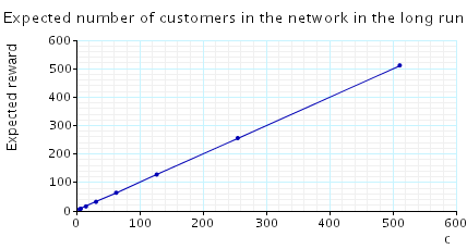
In the graph below we have plotted the results we checking the expected number of customers in the network in the long run.
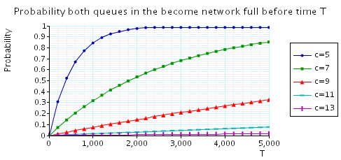
The probability that, from the initial state, the tandem network becomes fully occupied within T time units. The table and graph below presents the statistics and results when verifying this property.
| c: | T=2: | |||||
| Iters: | Time per iter: (s) | |||||
| MTBDD | Sparse | Hybrid | ||||
| 5 | 225 | 0.001120 | < 0.00001 | < 0.00001 | ||
| 7 | 241 | 0.001780 | 0.000000 | 0.000008 | ||
| 15 | 306 | 0.008987 | 0.000016 | 0.000033 | ||
| 31 | 437 | 0.022659 | 0.000080 | 0.000135 | ||
| 63 | 723 | 0.042553 | 0.000372 | 0.000564 | ||
| 127 | 1,325 | 0.094658 | 0.002080 | 0.002654 | ||
| 255 | 2,483 | 0.256095 | 0.014267 | 0.027096 | ||
| 511 | 4,733 | 0.786130 | 0.045681 | 0.081702 | ||
| 1,023 | 9,137 | 2.564898 | 0.119471 | 0.254866 | ||
| 2,047 | 17,814 | 9.097987 | 0.433326 | 0.899096 | ||
| 4,095 | 34,980 | - | - | 3.485094 | ||
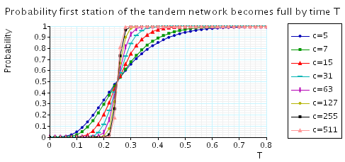
The probability that, from the initial state, the first station of the tandem network becomes fully occupied within T time units. The table and graph below presents the statistics and results when verifying this property.
| c: | T=0.5: | |||||
| Iters: | Time per iter: (s) | |||||
| MTBDD | Sparse | Hybrid | ||||
| 5 | 30 | 0.000900 | < 0.00001 | < 0.00001 | ||
| 7 | 30 | 0.001433 | < 0.00001 | < 0.00001 | ||
| 15 | 35 | 0.004743 | 0.000057 | 0.000057 | ||
| 31 | 50 | 0.008660 | 0.000260 | 0.000280 | ||
| 63 | 82 | 0.011988 | 0.001354 | 0.001476 | ||
| 127 | 148 | 0.017135 | 0.006176 | 0.006743 | ||
| 255 | 281 | 0.021281 | 0.027103 | 0.029299 | ||
| 511 | 545 | 0.033506 | 0.111947 | 0.123903 | ||
| 1,023 | 1,073 | 0.044320 | 0.410707 | 0.488582 | ||
| 2,047 | 2,125 | 0.112301 | 1.647587 | 1.972453 | ||
| 4,095 | 4,225 | 0.149460 | - | 8.087538 | ||
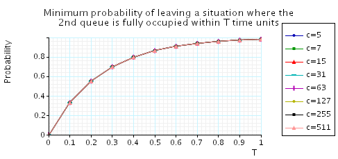
The minimum probability of leaving a situation where the second queue is fully occupied within T time units. The table and graph below presents the statistics and results when verifying this property.
| c: | T=0.5: | |||||
| Iters: | Time per iter: (s) | |||||
| MTBDD | Sparse | Hybrid | ||||
| 5 | 69 | 0.000058 | < 0.00001 | < 0.00001 | ||
| 7 | 92 | 0.000098 | < 0.00001 | < 0.00001 | ||
| 15 | 176 | 0.000125 | 0.000011 | < 0.00001 | ||
| 31 | 237 | 0.000139 | 0.000025 | 0.000030 | ||
| 63 | 302 | 0.000172 | 0.000086 | 0.000086 | ||
| 127 | 433 | 0.000219 | 0.000621 | 0.000672 | ||
| 255 | 718 | 0.000252 | 0.002249 | 0.002592 | ||
| 511 | 1,320 | 0.000309 | 0.010255 | 0.009667 | ||
| 1,023 | 2,479 | 0.000336 | 0.025934 | 0.041160 | ||
| 2,047 | 4,728 | 0.000355 | 0.098713 | 0.160120 | ||
| 4,095 | 9,133 | 0.000384 | 0.371677 | 0.626650 | ||
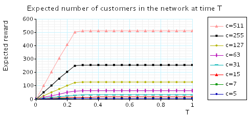
The expected number of customers in the network at time T. The table and graph below presents the statistics and results when verifying this property.
| c: | T=1: | |||||
| Iters: | Time per iter: (s) | |||||
| MTBDD | Sparse | Hybrid | ||||
| 5 | 198 | 0.001131 | < 0.00001 | < 0.00001 | ||
| 7 | 206 | 0.001801 | 0.000000 | 0.000010 | ||
| 15 | 239 | 0.006971 | 0.000017 | 0.000033 | ||
| 31 | 304 | 0.033102 | 0.000066 | 0.000109 | ||
| 63 | 435 | 0.075993 | 0.000260 | 0.000444 | ||
| 127 | 720 | 0.727625 | 0.001549 | 0.002162 | ||
| 255 | 1,323 | 1.212686 | 0.006620 | 0.009642 | ||
| 511 | 2,481 | 20.34883 | 0.026343 | 0.040297 | ||
| 1,023 | 1,063 | - | 0.067043 | 0.149812 | ||
| 2,047 | 2,111 | - | 0.267248 | 0.605698 | ||