(von Neumann)
Related publications: [NPKS05]
The case study concerns NAND multiplexing, a technique for constructing reliable computation from unreliable devices. As we move from deep submicron technology to nanotechnology for device manufacture, the need for architectures to be defect-tolerant is gaining importance. This is because, at the nanoscale, devices will be prone to errors due to manufacturing defects, ageing, and transient faults. Micro-architects will be required to design their logic around defect tolerance through redundancy.
In 1952, von Neumann studied the problem of constructing reliable computation from unreliable devices (due to unreliable valve based computers at that time), introducing a redundancy technique called NAND multiplexing [vN56]. He showed that, if the failure probabilities of the gates are sufficiently small and failures are statistically independent, then computations may be done with a high probability of correctness. Later, in [DO77], it was shown that a logarithmic redundancy is necessary for some Boolean function computations, and sufficient for all Boolean functions. In [Pip88], Pippenger showed that von Neumann's construction works only when the probability of failure per gate has a limit strictly less than 1/2, and that computation in the presence of noise (which can be seen as the presence of defect), requires more layers of redundancy. In [HJ02, NSF01], von Neumann's NAND multiplexing was compared to other techniques for fault-tolerance (such as R-fold Modular Redundancy and Reconfiguration) and some theoretical calculations were done to show that the redundancy level must be quite high to obtain acceptable levels of reliability.
The basic technique of multiplexing is to replace a processing unit by multiplexed units which have N copies of every input and output of the unit. In each multiplexing unit, there are N devices which in parallel process the copies of the inputs to give N outputs which represent the output of the original processing unit. If the inputs and devices are reliable, then each element of the output set should be identical and equal to the output of the corresponding processing unit. However, in the case when there are errors in the inputs and errors due to faulty devices, the outputs will not all take the same value. Instead, after defining some critical level Δ ∈ (0,0.5), the output of the multiplexing unit is considered to be stimulated (taking logical value true or `1') if at least (1 - Δ) ⋅ N of the outputs are stimulated and non-stimulated (taking logical value false or `0') if no more than Δ ⋅ N lines are stimulated. In cases where the number of stimulated outputs does not meet either of these criteria, that is, the number of stimulated outputs is in the interval (Δ ⋅ N , (1 - Δ)⋅ N), then the output is undecided, and hence a malfunction will occur.
The basic design of a multiplexing unit consists of two stages: the executive stage and the restorative stage. The executive stage carries out the basic function of the performance unit to be replaced, while the restorative stage is used to reduce the degradation in the executive stage caused by errors in both the inputs and the faulty devices.
We now consider multiplexing in the case when the processing unit is a single NAND gate. We therefore replace both the inputs and output of the gate with N copies and in the executive stage duplicate the NAND gate N times, as shown below.
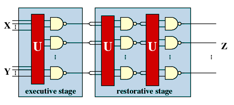
The unit U represents a random permutation of the input signals, that is, each signal of the first input is randomly paired with a signal from the second input to form an input pair for one of the copies of the NAND gate. Also shown in the figure is the restorative stage which is made using the same technique as the executive stage duplicating the outputs of the executive stage to use as its inputs. Note that, applying this approach only once will invert the result, therefore two steps are required. To give a more effective restoration mechanism the restorative stage can be iterated [vN56].
In [vN56], von Neumann concluded that, for extremely large N, the number of stimulated outputs of the executive stage is a stochastic variable, approximately normally distributed, and he gave an upper bound of 0.0107 for the probability of gate failure that can be tolerated. In other words, according to von Neumann, if the failure probability is greater than this threshold, then the probability of the NAND multiplexing system failing will be larger than a fixed, positive lower bound, no matter how large a bundle size is used. Recently, it was shown that, if each NAND gate fails independently, the tolerable threshold probability of each gate will be 0.08856 [EP98].
We now explain the PRISM model of von Neumann's NAND multiplexing system. We first note that it was during this phase that we noticed the error made by [HJ02] in modelling the random permutation made by the unit U. In the analysis technique of [HJ02] the random permutation made by U is instead modelled by a random choice with replacement. More precisely, in the approach of [HJ02], if in the previous stage there are k stimulated outputs, then after passing through the unit U the probability that any one of the resulting inputs of the current stage is stimulated is k/N.
As our analysis will demonstrate, these different approaches to modelling the unit U will lead to different conclusions about the reliability of the system under study. We should note however, that, as the bundle size increases, the differences between the results obtained by these different approaches will converge and, in fact, if the bundle sizes were infinite then these approaches would be equivalent. This can be seen in our results where the difference between the two approaches when the bundle size 20 is greater than when the bundle size is 40.
The first approach to modelling NAND multiplexing in PRISM was to directly model the system given in the figure above: for each stage construct a PRISM module for each of the N NAND gates in the stage and then combine these modules through synchronous parallel composition. However, this approach leads to the well know state space explosion problem. For example, if I/O bundle size equals 20, then just modelling the executive stage of the NAND multiplexing unit required more than 1.0e+14 states.
The important observation, which allowed us to overcome this problem, was that the actual value of each input and output is not important: instead one need only store the total number of stimulated (and non-stimulated) inputs and outputs. Furthermore, to allow us to compute these values, without having to store all the outputs of the NAND gates in each stage, we replace the set of N NAND gates working in parallel with N NAND gates working in sequence. This allows us to fold space into time, or in other words reuse the same NAND gate over time rather than making redundancy over space. We also apply the same methodology to the stages, that is, reuse the same module for each of the stages while keeping a record of the outputs from the previous stage.
Following these observations, the PRISM description of the NAND multiplexing system, for the case when the bundle size equals 20, is given in below. Note that taking this approach does not influence the performance of the system since each NAND gates works independently and the probability of each NAND gate failing is also independent.
// nand multiplex system
// gxn/dxp 20/03/03

// U (correctly) performs a random permutation of the outputs of the previous stage

dtmc

const int N; // number of inputs in each bundle
const int K; // number of restorative stages

const int M = 2*K+1; // total number of multiplexing units

// parameters taken from the following paper
// A system architecture solution for unreliable nanoelectric devices
// J. Han & P. Jonker
// IEEEE trans. on nanotechnology vol 1(4) 2002

const double perr = 0.02; // probability nand works correctly
const double prob1 = 0.9; // probability initial inputs are stimulated

// model whole system as a single module by resuing variables
// to decrease the state space
module multiplex

	u : [1..M]; // number of stages
	c : [0..N]; // counter (number of copies of the nand done)

	s : [0..4]; // local state
	// 0 - initial state
	// 1 - set x inputs
	// 2 - set y inputs
	// 3 - set outputs
	// 4 - done

	z : [0..N]; // number of new outputs equal to 1
	zx : [0..N]; // number of old outputs equal to 1
	zy : [0..N]; // need second copy for y
	// initially 9 since initially probability of stimulated state is 0.9

	x : [0..1]; // value of first input
	y : [0..1]; // value of second input

	[] s=0 & (c<N) -> (s'=1); // do next nand if have not done N yet
	[] s=0 & (c=N) & (u<M) -> (s'=1) & (zx'=z) & (zy'=z) & (z'=0) & (u'=u+1) & (c'=0); // move on to next u if not finished
	[] s=0 & (c=N) & (u=M) -> (s'=4) & (zx'=0) & (zy'=0) & (x'=0) & (y'=0); // finished (so reset variables not needed to reduce state space)

	// choose x permute selection (have zx stimulated inputs)
	// note only need y to be random
	[] s=1 & u=1  -> prob1 : (x'=1) & (s'=2) + (1-prob1) : (x'=0) & (s'=2); // initially random
	[] s=1 & u>1 & zx>0 -> (x'=1) & (s'=2) & (zx'=zx-1);
	[] s=1 & u>1 & zx=0 -> (x'=0) & (s'=2);

	// choose x randomly from selection (have zy stimulated inputs)
	[] s=2 & u=1 -> prob1 : (y'=1) & (s'=3) + (1-prob1) : (y'=0) & (s'=3); // initially random
	[] s=2 & u>1 & zy<(N-c) & zy>0  -> zy/(N-c) : (y'=1) & (s'=3) & (zy'=zy-1) + 1-(zy/(N-c)) : (y'=0) & (s'=3);
	[] s=2 & u>1 & zy=(N-c) & c<N -> 1 : (y'=1) & (s'=3) & (zy'=zy-1);
	[] s=2 & u>1 & zy=0 -> 1 : (y'=0) & (s'=3);

	// use nand gate
	[] s=3 & z<N & c<N -> (1-perr) : (z'=z+(1-x*y)) & (s'=0) & (c'=c+1) & (x'=0) & (y'=0) // not faulty
	         + perr    : (z'=z+(x*y))    & (s'=0) & (c'=c+1) & (x'=0) & (y'=0); // von neumann fault
	// [] s=3 & z<N -> (1-perr) : (z'=z+(1-x*y)) & (s'=0) & (c'=c+1) & (x'=0) & (y'=0) // not faulty
	//         + perr    : (z'=z+(x*y))    & (s'=0) & (c'=c+1) & (x'=0) & (y'=0); // von neumann fault

	[] s=4 -> true;

endmodule

// rewards: final value of gate
rewards
	[] s=0 & (c=N) & (u=M) : z/N;
endrewards
In the PRISM model given above we have assumed that the inputs X and Y are identically distributed (with probability 0.9 of being stimulated), and the NAND gates suffer from a von Neumann fault (inverted output) with probability 0.02. Note that, in the executive stage, a random permutation of the inputs cannot be performed as we only know the probability of each individual input being stimulated. However, for a fixed initial input, one can easily modify the PRISM model so that the system performs a random permutation of the input. To change the number of restorative stages, bundle size, input probabilities or probability of the NAND gates failing requires only modification of the constants given at the start of the description.
To model the approach of [HJ02], the only modifications that need to be made are to the probabilities with which the variables x and y are set (when the local state s equals 1 and 2 respectively), that is, replace the random permutation of the inputs with a random choice with replacement.
The tables below shows statistics and construction times of the models when the probability of gate failure equals 0.02. The tables include:
We also give the same statistics when the random permutation performed by the unit U is replaced by a random choice with replacement as used by [HJ02]. The results corresponding to this case are referenced 'UR', and we use 'U' to reference the results corresponding to the case when U does indeed perform a random permutation.
bundle size (N) equals 20
| Restorative stages: | U (random permutation) | UR (random choice with replacement) | ||||||||||
| States: | Nodes: | Leaves: | Construction: | States: | Nodes: | Leaves: | Construction: | |||||
| Time (s): | Iter.s: | Time (s): | Iter.s: | |||||||||
| 1 | 78,311 | 20,838 | 131 | 1.373 | 241 | 69,741 | 1,730 | 23 | 0.21 | 241 | ||
| 2 | 154,921 | 20,847 | 131 | 2.53 | 401 | 137,781 | 1,739 | 23 | 0.32 | 401 | ||
| 3 | 231,531 | 20,848 | 131 | 3.706 | 561 | 205,821 | 1,740 | 23 | 0.44 | 561 | ||
| 4 | 308,141 | 20,856 | 131 | 4.846 | 721 | 273,861 | 1,748 | 23 | 0.56 | 721 | ||
| 5 | 384,751 | 20,856 | 131 | 6.093 | 881 | 341,901 | 1,748 | 23 | 0.67 | 881 | ||
| 6 | 461,361 | 20,857 | 131 | 7.279 | 1041 | 409,941 | 1,749 | 23 | 0.81 | 1041 | ||
| 7 | 537,971 | 20,857 | 131 | 8.511 | 1201 | 477,981 | 1,749 | 23 | 0.90 | 1201 | ||
| 8 | 614,581 | 20,865 | 131 | 9.598 | 1361 | 546,021 | 1,757 | 23 | 1.07 | 1361 | ||
| 9 | 691,191 | 20,865 | 131 | 10.94 | 1521 | 614,061 | 1,757 | 23 | 1.19 | 1521 | ||
| 10 | 767,801 | 20,865 | 131 | 11.98 | 1681 | 682,101 | 1,757 | 23 | 1.27 | 1681 | ||
| 11 | 844,411 | 20,865 | 131 | 13.44 | 1841 | 750,141 | 1,757 | 23 | 1.45 | 1841 | ||
| 12 | 921,021 | 20,866 | 131 | 14.43 | 2001 | 818,181 | 1,758 | 23 | 1.53 | 2001 | ||
| 13 | 997,631 | 20,866 | 131 | 16.01 | 2161 | 886,221 | 1,758 | 23 | 1.65 | 2161 | ||
bundle size (N) equals 40
| Restorative stages: | U (random permutation) | UR (random choice with replacement) | ||||||||||
| States: | Nodes: | Leaves: | Construction: | States: | Nodes: | Leaves: | Construction: | |||||
| Time (s): | Iter.s: | Time (s): | Iter.s: | |||||||||
| 1 | 1,004,821 | 46,221 | 898 | 5.42 | 481 | 534,681 | 3,262 | 43 | 0.61 | 481 | ||
| 2 | 2,003,041 | 46,230 | 898 | 9.97 | 801 | 1,062,761 | 3,271 | 43 | 1.00 | 801 | ||
| 3 | 3,001,261 | 46,231 | 898 | 16.4 | 1,121 | 1,590,841 | 3,272 | 43 | 1.45 | 1,121 | ||
| 4 | 3,999,481 | 46,239 | 898 | 20.5 | 1,441 | 2,118,921 | 3,280 | 43 | 2.03 | 1,441 | ||
| 5 | 4,997,701 | 46,239 | 898 | 24.2 | 1,761 | 2,647,001 | 3,280 | 43 | 2.44 | 1,761 | ||
| 6 | 5,995,921 | 46,240 | 898 | 30.7 | 2,081 | 3,175,081 | 3,281 | 43 | 2.69 | 2,081 | ||
| 7 | 6,994,141 | 46,240 | 898 | 35.1 | 2,401 | 3,703,161 | 3,281 | 43 | 3.96 | 2,401 | ||
bundle size (N) equals 60
| Restorative stages: | U (random permutation) | UR (random choice with replacement) | ||||||||||
| States: | Nodes: | Leaves: | Construction: | States: | Nodes: | Leaves: | Construction: | |||||
| Time (s): | Iter.s: | Time (s): | Iter.s: | |||||||||
| 1 | 4,717,531 | 100,443 | 2,421 | 11.7 | 721 | 1,778,821 | 4,328 | 63 | 1.91 | 721 | ||
| 2 | 9,420,361 | 100,452 | 2,421 | 27.9 | 1,201 | 3,542,941 | 4,337 | 63 | 2.15 | 1,201 | ||
| 3 | 14,123,191 | 100,453 | 2,421 | 37.4 | 1,681 | 5,307,061 | 4,338 | 63 | 2.59 | 1,681 | ||
| 4 | 18,826,021 | 100,461 | 2,421 | 52.8 | 2,161 | 7,071,181 | 4,346 | 63 | 3.58 | 2,161 | ||
| 5 | 23,528,851 | 100,461 | 2,421 | 62.0 | 2,641 | 8,835,301 | 4,346 | 63 | 4.62 | 2,641 | ||
| 6 | 28,231,681 | 100,462 | 2,421 | 78.8 | 3,121 | 10,599,421 | 4,347 | 63 | 4.96 | 3,121 | ||
| 7 | 32,934,511 | 100,462 | 2,421 | 99.2 | 3,601 | 12,363,541 | 4,347 | 63 | 5.74 | 3,601 | ||
The properties we consider are the probability of there being k stimulated outputs (which in terms of the PRISM model presented in above, corresponds to the probability of reaching the state where z=k, u=3 and c=20), for k=0,...,N where N is the system's I/O bundle size. By performing this analysis we have in fact computed the output distribution of the system, and hence any measure of reliability can be calculated from these results. Note that PRISM can be used directly for computing these measures of reliability, for example, the probability of errors being less than than k% and the expected number of incorrect outputs of the system.
The model checking statistics given below are for calculating the probability of there being 0 stimulated outputs when the probability of gate failure equals 0.01 using PRISm's hybrid engine.
There are two precomputation steps in the model checking procedure involving BDD based fixpoint algorithms: Prob1 and Prob0 which finds those states such that the probability of satisfying the formula is 1 and 0 respectively.
In the main algorithm we stop iterating when the relative error between subsequent iteration vectors is less than 1e-6, that is:

bundle size (N) equals 20
| Restorative stages: | U (random permutation) | UR (random choice with replacement) | ||||||||
| Time: | Iterations: | Time: | Iterations: | |||||||
| Prob1: | Prob0: | Main: | Prob1: | Prob0: | Main: | |||||
| 1 | 3.29 | 246 | 241 | 2 | 0.411 | 246 | 241 | 2 | ||
| 2 | 5.30 | 406 | 401 | 2 | 0.779 | 406 | 401 | 2 | ||
| 3 | 7.61 | 566 | 561 | 2 | 1.091 | 566 | 561 | 2 | ||
| 4 | 9.71 | 726 | 721 | 2 | 1.521 | 726 | 721 | 2 | ||
| 5 | 12.3 | 886 | 881 | 2 | 1.862 | 886 | 881 | 2 | ||
| 6 | 14.6 | 1,046 | 1,041 | 2 | 2.19 | 1,046 | 1,041 | 2 | ||
| 7 | 16.0 | 1,206 | 1,201 | 2 | 2.42 | 1,206 | 1,201 | 2 | ||
| 8 | 19.2 | 1,366 | 1,361 | 2 | 2.72 | 1,366 | 1,361 | 2 | ||
| 9 | 21.1 | 1,526 | 1,521 | 2 | 3.11 | 1,526 | 1,521 | 2 | ||
| 10 | 23.9 | 1,686 | 1,681 | 2 | 3.44 | 1,686 | 1,681 | 2 | ||
| 11 | 27.8 | 1,846 | 1,841 | 2 | 4.00 | 1,846 | 1,841 | 2 | ||
| 12 | 28.9 | 2,006 | 2,001 | 2 | 4.39 | 2,006 | 2,001 | 2 | ||
| 13 | 32.0 | 2,166 | 2,161 | 2 | 4.55 | 2,166 | 2,161 | 2 | ||
bundle size (N) equals 40
| Restorative stages: | U (random permutation) | UR (random choice with replacement) | ||||||||
| Time: | Iterations: | Time: | Iterations: | |||||||
| Prob1: | Prob0: | Main: | Prob1: | Prob0: | Main: | |||||
| 1 | 28.4 | 486 | 481 | 2 | 2.78 | 486 | 481 | 2 | ||
| 2 | 46.1 | 806 | 801 | 2 | 4.53 | 806 | 801 | 2 | ||
| 3 | 64.3 | 1,126 | 1,121 | 2 | 5.90 | 1,126 | 1,121 | 2 | ||
| 4 | 76.1 | 1,446 | 1,441 | 2 | 7.19 | 1,446 | 1,441 | 2 | ||
| 5 | 88.3 | 1,766 | 1,761 | 2 | 9.93 | 1,766 | 1,761 | 2 | ||
| 6 | 118 | 2,086 | 2,081 | 2 | 12.4 | 2,086 | 2,081 | 2 | ||
| 7 | 130 | 2,406 | 2,401 | 2 | 13.6 | 2,406 | 2,401 | 2 | ||
bundle size (N) equals 40
| Restorative stages: | U (random permutation) | UR (random choice with replacement) | ||||||||
| Time: | Iterations: | Time: | Iterations: | |||||||
| Prob1: | Prob0: | Main: | Prob1: | Prob0: | Main: | |||||
| 1 | 48.7 | 726 | 721 | 2 | 3.88 | 726 | 721 | 2 | ||
| 2 | 97.1 | 1,206 | 1,201 | 2 | 10.6 | 1,206 | 1,201 | 2 | ||
| 3 | 140 | 1,686 | 1,681 | 2 | 13.6 | 1,686 | 1,681 | 2 | ||
| 4 | 170 | 2,166 | 2,161 | 2 | 17.4 | 2,166 | 2,161 | 2 | ||
| 5 | 254 | 2,646 | 2,641 | 2 | 20.8 | 2,646 | 2,641 | 2 | ||
| 6 | 427 | 3,126 | 3,121 | 2 | 22.7 | 3,126 | 3,121 | 2 | ||
| 7 | 608 | 3,606 | 3,601 | 2 | 24.2 | 3,606 | 3,601 | 2 | ||
We now study the performance of NAND multiplexing systems both when the I/O bundles are of size 20, 40 and 60. In all the experiments, we assume that the inputs X and Y are identical (this is often true in circuits containing similar devices) and that initially 90% of the inputs are stimulated (correct). We suppose that the gate failure in each NAND is a von Neumann fault, that is, when a gate fails, the value of its output is inverted.
Our analysis of the reliability of the NAND multiplexing system using probabilistic model checking concentrates on the effects of the failure probabilities of the NAND gates and of the number of restorative stages. Recall that, to change either of these in the PRISM language description of the system, one needs only change the parameter probz or the parameter M. The results we present show:
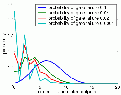
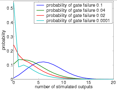
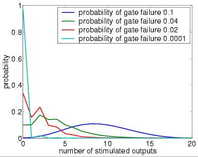
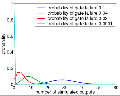
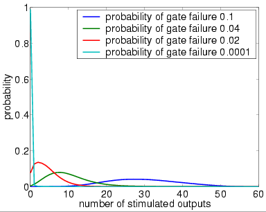
In graphs below we present, for systems with a different numbers of restorative stages and both in the case when the unit U performs a random permutation and when it performs a random choice with replacement, the output distribution when the probability of gate failure equals 0.1, 0.04, 0.02 and 0.0001.
Note that the system is supposed to model a correctly functioning NAND gate and we assume that the inputs are correct when stimulated. Hence, the more outputs that are non-stimulated, the greater the reliability of the system.
1 restorative stage (random permutation)
1 restorative stage (random choice with replacement)
4 restorative stages (random permutation)
4 restorative stages (random choice with replacement)
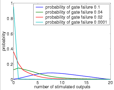
7 restorative stages (random permutation)
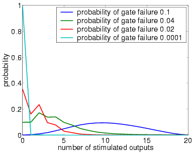
7 restorative stages (random choice with replacement)
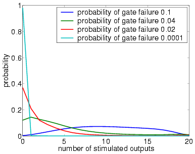
In graphs below we present, for systems with a different numbers of stages and both in the case when the unit U performs a random permutation and when it performs a random choice with replacement, the output distribution when the probability of gate failure equals 0.1, 0.04, 0.02 and 0.0001.
Note that the system is supposed to model a correctly functioning NAND gate and we assume that the inputs are correct when stimulated. Hence, the more outputs that are non-stimulated, the greater the reliability of the system.
1 restorative stage (random permutation)
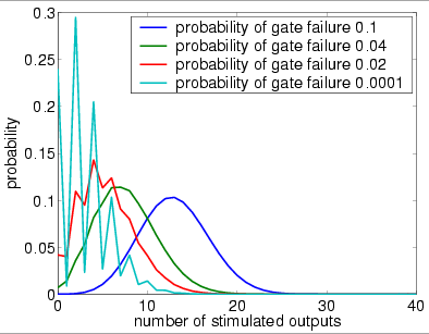
1 restorative stage (random choice with replacement)
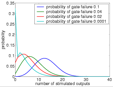
4 restorative stages (random permutation)
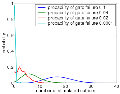
4 restorative stages (random choice with replacement)
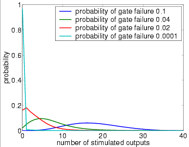
7 restorative stages (random permutation)
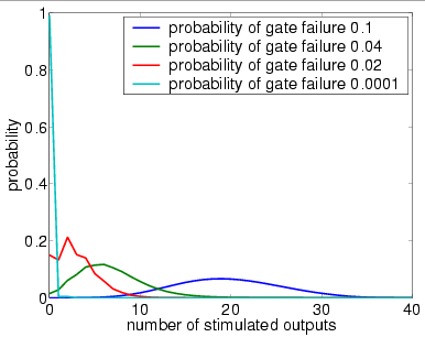
7 restorative stages (random choice with replacement)
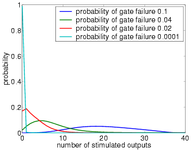
In graphs below we present, for systems with a different numbers of stages and both in the case when the unit U performs a random permutation and when it performs a random choice with replacement, the output distribution when the probability of gate failure equals 0.1, 0.04, 0.02 and 0.0001.
Note that the system is supposed to model a correctly functioning NAND gate and we assume that the inputs are correct when stimulated. Hence, the more outputs that are non-stimulated, the greater the reliability of the system.
1 restorative stage (random permutation)
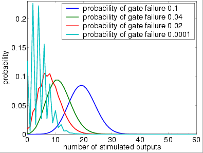
1 restorative stage (random choice with replacement)
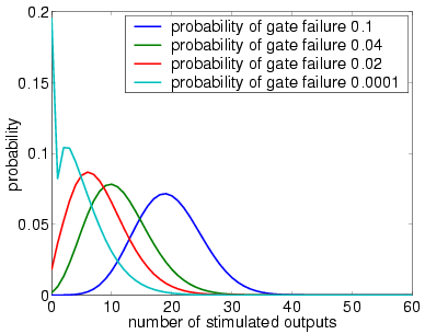
4 restorative stages (random permutation)

4 restorative stages (random choice with replacement)
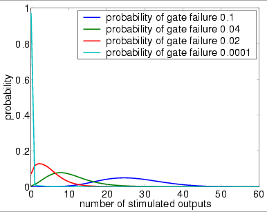
7 restorative stages (random permutation)
7 restorative stages (random choice with replacement)
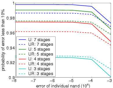
The following graph plots the probability that at most 10% of the outputs of the overall system are incorrect (stimulated) against the failure probability of the gates.
bundle size (N) equals 20
bundle size (N) equals 40
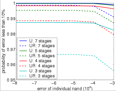
bundle size (N) equals 60
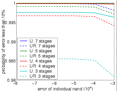
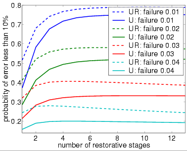
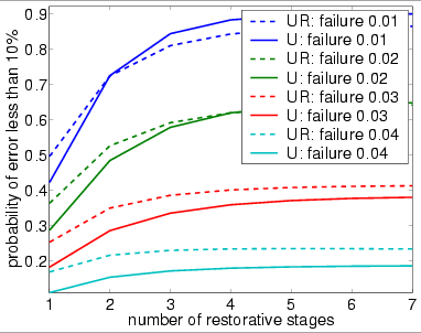
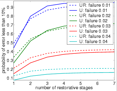
The following graph plots the probability that at most 10% of the outputs of the overall system are incorrect (stimulated) against the number of stages of the system.
bundle size (N) equals 20
bundle size (N) equals 40
bundle size (N) equals 60
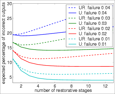
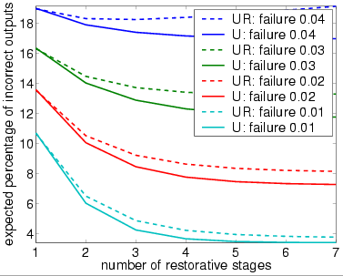
The following graph plots the expected percentage of incorrect (stimulated) inputs against the number of stages of the system.
bundle size N equals 20
bundle size N equals 40
bundle size N equals 60
