
In this case study we investigate the likelihood that a pair of nodes are connected in a random graph. More precisely, we consider the set of random graphs G(n,p), i.e. the set of random graphs with n nodes where the probability of there being an edge between any two nodes equals p. We examine whether a graph G is ''1-2 connected'', i.e. whether there exists a path from node 1 to node 2.
To model this problem in PRISM we split the modelling into two stages. In the first stage, we (randomly) construct a graph from G(n,p). In the second stage, we find all nodes that can reach node 2, and hence find whether node 1 can reach node 2. More precisely, in the second stage, we find nodes that have a path to node 2 by searching for nodes for which one can reach (in one step) a node for which we have already found the existence of a path to node 2. Note that, because the above may hold for a set of nodes we make a non-deterministic choice as to which node we choose to consider first. Hence, the model is an MDP.
Below we give the PRISM code for in the case when n equals 4.
// checking for a path between nodes 1 and 2 for random graphs ($ nodes)
// gxn/dxp 12/11/04

mdp

const double p; // probability there exists an edge between two nodes

// program counter (decides which edge is set randomly next)
// note: the second modelling stage does not start until the program
// counter has reached its maximum value, i.e. the random graph has
// been constructed
module PC

	pc : [0..12];

	[s12] pc=0 -> (pc'=pc+1);
	[s13] pc=1 -> (pc'=pc+1);
	[s14] pc=2 -> (pc'=pc+1);
	[s23] pc=3 -> (pc'=pc+1);
	[s24] pc=4 -> (pc'=pc+1);
	[s34] pc=5 -> (pc'=pc+1);

endmodule

// module for path between 1 and 2
module M12

	x12 : bool;

	// randomly decide if there exists an edge
	[s12] true -> p:(x12'=true)+(1-p):(x12'=false);
	// update if we can find a path to 2
	[] pc=6 & !x12 & (false | (x13 & x23) | (x14 & x24)) -> (x12'=true);

endmodule

// module for path between 1 and 3
module M13

	x13 : bool;

	// randomly decide if there exists an edge
	[s13] true -> p:(x13'=true)+(1-p):(x13'=false);

endmodule

// module for path between 1 and 4
module M14

	x14 : bool;

	// randomly decide if there exists an edge
	[s14] true -> p:(x14'=true)+(1-p):(x14'=false);

endmodule

// module for path between 2 and 3
module M23

	x23 : bool;

	// randomly decide if there exists an edge
	[s23] true -> p:(x23'=true)+(1-p):(x23'=false);
	// update if we can find a path to 2
	[] pc=6  & !x23 & (false | (x12 & x13) | (x24 & x34)) -> (x23'=true);

endmodule

// module for path between 3 and 4
module M24

	x24 : bool;

	// randomly decide if there exists an edge
	[s24] true -> p:(x24'=true)+(1-p):(x24'=false);
	// update if we can find a path to 2
	[] pc=6  & !x24 & (false | (x12 & x14) | (x23 & x34)) -> (x24'=true);

endmodule

// module for path between 3 and 4
module M34

	x34 : bool;

	// randomly decide if there exists an edge
	[s34] true -> p:(x34'=true)+(1-p):(x34'=false);

endmodule
The table below shows statistics for models we have built for random graphs with different numbers of nodes (different values of n). Note that these statistics are identical for all values of p, expect for the special cases when p equals 0, 0.5 or 1. The tables include:
| n: | Model: | MTBDD: | Construction: | |||||
| States: | Nodes: | Leaves: | Time (s): | Iter.s: | ||||
| 2 | 3 | 18 | 4 | 0.063 | 2 | |||
| 3 | 15 | 86 | 4 | 0.071 | 4 | |||
| 4 | 127 | 291 | 4 | 0.098 | 7 | |||
| 5 | 2,047 | 732 | 4 | 0.120 | 11 | |||
| 6 | 65,535 | 1,629 | 4 | 0.149 | 16 | |||
| 7 | 194,303 | 3,664 | 4 | 0.284 | 22 | |||
| 8 | 536,870,911 | 8,234 | 4 | 0.455 | 29 | |||
| 9 | 137,438,953,471 | 19,079 | 4 | 0.915 | 37 | |||
| 10 | 70,368,744,177,663 | 32,119 | 4 | 2.52 | 46 | |||
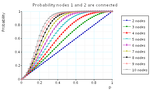
To find the probability that the nodes 1 and 2 are connected we verify the property: Pmax=?[true U x12].
The following graph plots, for the cases when n=2,3,...,10, this probability as the value of p varies.
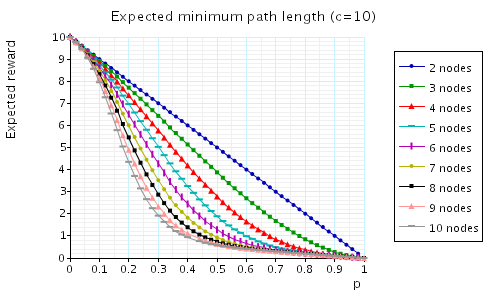
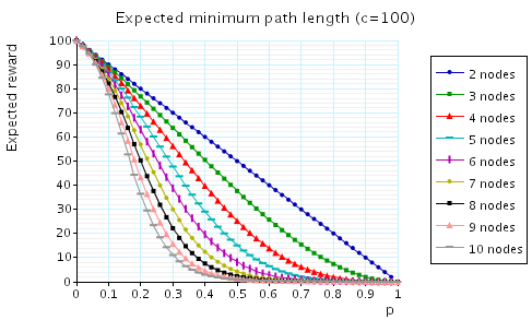
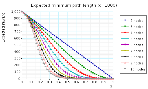
In addition, we have calculated the expected shortest path between 1 and 2. To treat the cases when the nodes 1 and 2 are not connected, we set the path length to be c when no path between 1 and 2 exists.
Each of the following graphs plot, for the cases when n=2,3,...,10, the expected shortest path between 1 and 2 as the value of p varies. The difference between the graphs is the value we assign c, that is the cost associated with a graph when the nodes 1 and 2 are not connected.