

This example illustrates the use of Markov decision processes to solve a simple probabilistic planning problem.
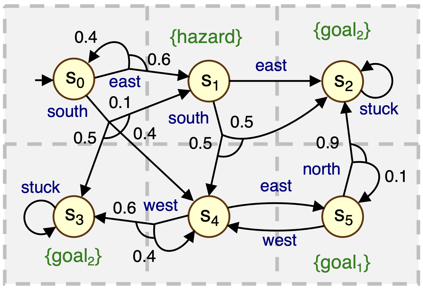
We consider a robot moving through a 3 x 2 grid. Here is a graphical illustration of the robot and its possible behaviours in the environment:
The PRISM code to model the robot is shown below.
// MDP model of a robot moving through
// terrain that is divided up into a 3×2 grid

mdp

module robot

	s : [0..5] init 0; // Current grid location

	[east] s=0 -> 0.6 : (s'=1) + 0.4 : (s'=0);
	[south] s=0 -> 0.4 : (s'=4) + 0.1 : (s'=1) + 0.5 : (s'=3);
	[east] s=1 -> 1 : (s'=2);
	[south] s=1 -> 0.5 : (s'=4) + 0.5 : (s'=2);
	[stuck] s=2 -> 1 : (s'=2);
	[stuck] s=3 -> 1 : (s'=3);
	[east] s=4 -> 1 : (s'=5);
	[west] s=4 -> 0.6 : (s'=3) + 0.4 : (s'=4);
	[north] s=5 -> 0.9 : (s'=2) + 0.1 : (s'=5);
	[west] s=5 -> 1 : (s'=4);

endmodule

// Atomic propositions labelling states

label "hazard" = s=1;
label "goal1" = s=5;
label "goal2" = s=2|s=3;

// Reward structures

// Number of moves between locations
rewards "moves"
	[north] true : 1;
	[east] true : 1;
	[south] true : 1;
	[west] true : 1;
endrewards
The first line indicates that this model is a Markov decision process (MDP). The remaining lines describe a single PRISM module, which we use to model the behaviour of the robot. We use one variable to represent the state of the system: s, denoting the current position of the robot in the 3 x 2 grid.
 If you are not yet familiar with the PRISM modelling language, read the sections on
modules/variables and
commands
in the manual to help clarify the model above.
If you are not yet familiar with the PRISM modelling language, read the sections on
modules/variables and
commands
in the manual to help clarify the model above.
Download the model file robot.prism for this example from the link above.
Launch the PRISM GUI
(click the shortcut on Windows or run bin/xprism elsewhere)
and load this file using the "Model | Open model" menu option.
You should see a green tick in the top left corner indicating that the model was loaded and parsed successfully.
Click on the "Simulator" tab at the bottom of the GUI.
You can now use the
simulator
to explore the model.
Create a new path by double-clicking on the main part of the window
(or right-clicking and selecting "New path").
Then, use the "Simulate" button repeatedly to generate a sample execution of the algorithm.
Look at the trace displayed in the main part of the window.
What is the final value of s?
Why is that?
Right-click and select "Reset path".
Then, step through a trace of the algorithm manually
by double-clicking the available transitions
from the "Manual exploration" box.
Try to reach the goal1-labelled state without passing through the hazard-labelled state
(the value of each label in the current state is shown in the top right of the window).
Now change the value of the "Steps" option under the "Simulate" button from 1 to 10
and, using the "Reset path" option and "Simulate" buttons,
generate several different random traces.
What is the minimum path length you observe? What is the maximum?
We will now use PRISM to analyse the model and extract optimal policies that yield the highest probability of satisfying a user-defined goal. (Note that in PRISM policies are referred to as "strategies")
Download the properties file robot.props below and then
load it into PRISM using the "Properties | Open properties list" menu option.
Pmax=? [ F "goal1" ]
The property is of the form Pmax=? [ F phi ] which, intuitively, means "what is the maximum probability under any policy, from the initial state of the MDP, of reaching a state where phi is true?"
From your knowledge about MDPs, what answer do you expect for the property above?
Right click on the property in the GUI and select "Verify".
Is the answer as you expected?
Click on the "Log" tab to see some additional information that PRISM has displayed regarding the calculations performed.
PRISM uses iterative numerical solution techniques which converge towards the correct result. The numerical computation process is terminated when it is detected that the answers have converged sufficiently. Have a look at the manual for more information.
Open the PRISM options panel from the menu.
Find the "Termination epsilon" parameter and change it from 1.0e-6 to 1.0e-10.
Re-verify the property and see how the answer changes.
Check the log again and see many more iterations were required.
Reset the "Termination epsilon" parameter to 1.0e-6.
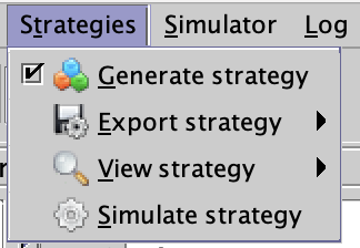
We now want to obtain the corresponding optimal policy for the robot, yielding this maximum probability of reaching goal1. For that, we tick the box "Generate Strategy" under the "Strategies" menu:
Now, after verifying the property again, we can extract the optimal policy by selecting "View Strategy" -> "Action List" under the "Strategies" tab. What is the optimal policy?
You can also generate some paths in the simulator, and the policy will be enforced/displayed at each step.
In the example above, the optimal policy is "memoryless", i.e., it only depends on the current state and not in any way on the history of previously visited states.
We now consider a second property:
const int k;

Pmax=? [ !"hazard" U<=k "goal2" ]
From your knowledge about MDPs and PCTL, what does the property mean?
Without using PRISM, what are the maximum probabilities and optimal policies
for the property with values k = 1,2,3?
Now check your answers for the previous part with PRISM. You can create a constant by right-clicking in the "Constants" panel below the properties and changing the default name provided. Similarly, to create a new property, right click in the properties panel. What does the output for the optimal policies look like and how do you interpret it? It may help to explore the policies in the simulator again.
Does the optimal policy change for different values of k? Explain.
[ Back to index ]