

This example concerns dynamic power management (DPM) schemes, which are sets of instructions used to switch between different power states of computing devices. This example is actually based on a specific case study from the literature [BBPM99], concerning an IBM TravelStar VP disk drive with 5 power states. However, in the following, we describe the DPM system in a fairly generic way.
The DPM system comprises several components:
The Service Provider (disk drive) has several different power states. The idea is that these states have different power consumptions but also different response times when a service is to be performed. Switches between power states are either performed by the Service Provider itself or initiated by the Power Manager. A good strategy for switching between these states will be one that keeps energy consumption as low as possible whilst maintaining an acceptable level of service.
Our initial PRISM model is the following:
dtmc

// Max size of service request queue
const int QMAX = 10;

//-------------------------------------------------------------------------

// Service Requester (SR)

module SR

	sr : [0..1] init 0;
	// 0 idle
	// 1 1req

	[tick] sr=0 -> 0.898: (sr'=0) + 0.102: (sr'=1);
	[tick] sr=1 -> 0.454: (sr'=0) + 0.546: (sr'=1);

endmodule

//-------------------------------------------------------------------------

// Service Queue (SQ)

module SQ

	q : [0..QMAX] init 0;

	// request removed by SP if it is active
	[tick] sr=0 & sp=0 -> (q'=max(q-1,0));
	[tick] sr=1 & sp=0 -> (q'=q);

	// otherwise do nothing
	[tick] sr=0 & sp>0 -> (q'=q);
	[tick] sr=1 & sp>0 & q<QMAX -> (q'=q+1);
	[tick] sr=1 & sp>0 & q=QMAX -> (q'=q);

endmodule

//-------------------------------------------------------------------------

// Service Provider (SP) (Disk drive)

module SP

	sp : [0..1] init 1;
	// 0 active
	// 1 idle

endmodule

//-------------------------------------------------------------------------

// Labels:

label "queue_full" = (q=QMAX);
label "queue_empty" = (q=0);

// Reward structures:

rewards "time"
	[tick] true : 1;
endrewards

rewards "queue"
	true : q;
endrewards
This model is a a discrete-time Markov chain (DTMC), like in the previous example. Later, we will adapt the model, making it a Markov decision process (MDP). Initially, we focus on just two components of the system: the Service Requester (SR) and the Service Queue (SQ). We will add the other components in due course. We also add a dummy Service Provider (SP) component for convenience.
The Service Requester has 2 states, idle and 1req, represented using a variable sr. When in state 1req, the SR sends one request per time step (1 ms). The probabilities of switching between these two states at each step, as shown in the model, were determined based on time-stamped traces of disk accesses measured on real machines.
The Service Queue comprises a single variable q, representing the number of requests waiting to be processed. At each step, a request is added to the queue if supplied by the SR (unless the queue is full, in which case the request is lost). Requests will be removed from the queue and processed by the Service Provider, assuming it is active (denoted by sp=0). For now, we assume that this is never the case.
 Take a look at the model and make sure you understand how it works.
The tick actions, included in square brackets at the start of each command,
indicate that the modules move simultaneously, using
synchronisation.
Notice also that modules are allowed to read (but not modify) the variables of other modules.
Take a look at the model and make sure you understand how it works.
The tick actions, included in square brackets at the start of each command,
indicate that the modules move simultaneously, using
synchronisation.
Notice also that modules are allowed to read (but not modify) the variables of other modules.
Download the model above, load it into PRISM and execute some paths through the model using the simulator.
You will see that there is also a label "queue_full" in the model,
indicating when the request queue becomes full.
Now move to the Properties tab in the PRISM GUI.
Create a new integer constant, named T
and then add the following property:
P=? [ F<=T "queue_full" ]
What does this mean? (See here if you want to see more details about the P operator.) Plot the value of this property for values of T between 0 and 250 (in steps of 10).
You will notice that the model also includes a reward structure that can be used to measure time.
Use PRISM to compute the expected time until the queue becomes full.
(You will need to use a property of the form
R{"time"}=? [ ... ]
rather than
R=? [ ... ]
since the model has more than one reward structure.
Lastly, try plotting the
"expected queue size at time T"
for values of T between 0 and 250
using the property:
R{"queue"}=? [ I=T ]
Are the results for these properties as you expected?
Remember that we have not actually modelled the Service Provider yet, just added a dummy module.
So, requests are generated but never dealt with.
Next, we add the Service Provider (SP) component, representing the disk drive. This has 5 different power modes: active, idle, idlelp (idle low power), stdby (on standby) and sleep. These, and the possible transitions between them, are shown in the figure below.
The SP will move between power states when it is instructed to do so by the power manager. Transitions between power states are not immediate, however, so our model includes additional "transient states" which, like in the Service Requester above, model a random delay.
The PRISM code below shows the module added to model the the SP component. The comments show the possible value of its sp variable: the main power states are represented by values 0, 1, 3, 6 and 9; the other values are for transient states. The transitions between power states of the SP will be controller by the Power Manager (PM) (more precisely, its variable pm). These transitions can be seen in the second part of the SP module. For now, we add a dummy PM module, which fixes pm=0.
// Service Provider (SP) (Disk drive)

module SP

	sp : [0..10] init 1;
	// 0 active
	// 1 idle
	// 2 active_idlelp
	// 3 idlelp
	// 4 idlelp_active
	// 5 active_stby
	// 6 stby
	// 7 stby_active
	// 8 active_sleep
	// 9 sleep
	// 10 sleep_active

	// states where PM has no control (transient states)
	[tick] sp=2  ->   0.75   : (sp'=2) + 0.25   : (sp'=3);  // active_idlelp
	[tick] sp=4  ->   0.25   : (sp'=0) + 0.75   : (sp'=4);  // idlelp_active
	[tick] sp=5  ->   0.995  : (sp'=5) + 0.005  : (sp'=6);  // active_stby
	[tick] sp=7  ->   0.005  : (sp'=0) + 0.995  : (sp'=7);  // stby_active
	[tick] sp=8  ->   0.9983 : (sp'=8) + 0.0017 : (sp'=9);  // active_sleep
	[tick] sp=10 ->   0.0017 : (sp'=0) + 0.9983 : (sp'=10); // sleep_active

	// states where PM has control
	// goto_active
	[tick] sp=0 & pm=0 -> (sp'=0); // active
	[tick] sp=1 & pm=0 -> (sp'=0); // idle
	[tick] sp=3 & pm=0 -> (sp'=4); // idlelp
	[tick] sp=6 & pm=0 -> (sp'=7); // stby
	[tick] sp=9 & pm=0 -> (sp'=10); // sleep
	// goto_idle
	[tick] sp=0 & pm=1 -> (sp'=1); // active
	[tick] sp=1 & pm=1 -> (sp'=1); // idle
	[tick] sp=3 & pm=1 -> (sp'=3); // idlelp
	[tick] sp=6 & pm=1 -> (sp'=6); // stby
	[tick] sp=9 & pm=1 -> (sp'=9); // sleep
	// goto_idlelp
	[tick] sp=0 & pm=2 -> (sp'=2); // active
	[tick] sp=1 & pm=2 -> (sp'=2); // idle
	[tick] sp=3 & pm=2 -> (sp'=3); // idlelp
	[tick] sp=6 & pm=2 -> (sp'=6); // stby
	[tick] sp=9 & pm=2 -> (sp'=9); // sleep
	// goto_stby
	[tick] sp=0 & pm=3 -> (sp'=5); // active
	[tick] sp=1 & pm=3 -> (sp'=5); // idle
	[tick] sp=3 & pm=3 -> (sp'=5); // idlelp
	[tick] sp=6 & pm=3 -> (sp'=6); // stby
	[tick] sp=9 & pm=3 -> (sp'=9); // sleep
	// goto_sleep
	[tick] sp=0 & pm=4 -> (sp'=8); // active
	[tick] sp=1 & pm=4 -> (sp'=8); // idle
	[tick] sp=3 & pm=4 -> (sp'=8); // idlelp
	[tick] sp=6 & pm=4 -> (sp'=8); // stby
	[tick] sp=9 & pm=4 -> (sp'=9); // sleep

endmodule

//-------------------------------------------------------------------------

// Power Manager (PM)

module PM

	pm : [0..4] init 0;
	// 0 - go to active
	// 1 - go to idle
	// 2 - go to idlelp
	// 3 - go to stby
	// 4 - go to sleep

endmodule
Remove the dummy SP module from your current model and paste in the code from above.
Now, re-plot the last property from above
("expected queue size at time T")
on the same graph that you produced earlier.
What effect does the new component have and why?
Use the simulator to generate some random traces if that helps.
Finally, we add the Power Manager (PM) component to the model. We will start with a very simple PM and then adapt it. In order to allow the PM to issue instructions to the SP, we will change the model so that it alternately makes two kinds of transitions: the first is a choice by the PM (action choose), the second is the tick action, used in the model so far. To enforce alternation of these types of actions, we add a special scheduler module (sched).
Remove the dummy PM module from your model and paste in the code below.
This simple Power Manager waits until the queue is full before switching on the Service Provider.
On a new graph, again plot the expected queue size over time
(a direct comparison with the models/graphs from above is not appropriate because we
have doubled the number of steps in the model by adding choose).
// Power Manager (PM)

module PM

	pm : [0..4] init 1;
	// 0 - go to active
	// 1 - go to idle
	// 2 - go to idlelp
	// 3 - go to stby
	// 4 - go to sleep

	// Only go to active when queue is full
	[choose] q=QMAX -> (pm'=0);
	[choose] q<QMAX -> (pm'=1);

	[tick] true -> (pm'=pm);

endmodule

//-------------------------------------------------------------------------

// Scheduler

module sched

	turn : [0..1];

	[choose] turn=0 -> (turn'=1);
	[tick] turn=1 -> (turn'=0);

endmodule
Now let's consider a few additional properties. In particular, we would like to examine the trade-off between the level of service provided by the system and the energy usage required to achieve it.
The expected queue size is just one indicator of the level of service provided.
Create another copy of the time
reward structure used earlier to count clock ticks and change it so that
it instead tracks the number of requests that get lost due to the queue being full.
Give it the name "lost"
and then use following property to compute the expected number of request lost as time passes.
(See here
for more details about reward structures.)
R{"lost"}=? [ C<=T ]
Using a similar property, then compute the expected energy usage over the same period.
Based on the real power usage figures for the disk drive in this case study,
the following reward structure can be used to compute energy usage.
rewards "energy"
	[tick] sp=0  : 2.5;
	[tick] sp=1  : 1.5;
	[tick] sp=2  : 2.5;
	[tick] sp=3  : 0.8;
	[tick] sp=4  : 2.5;
	[tick] sp=5  : 2.5;
	[tick] sp=6  : 0.3;
	[tick] sp=7  : 2.5;
	[tick] sp=8  : 2.5;
	[tick] sp=9  : 0.1;
	[tick] sp=10 : 2.5;
endrewards
Now, we'll design a better PM component.
Consider a randomised power management scheme which,
when the queue is anywhere between empty and full,
randomly chooses whether to move to active or idle
(but still chooses active or idle when the queue is full or empty, respectively).
Add a constant p
to the model which represents the probability of choosing active.
Now, modify the PM module to work as described above.
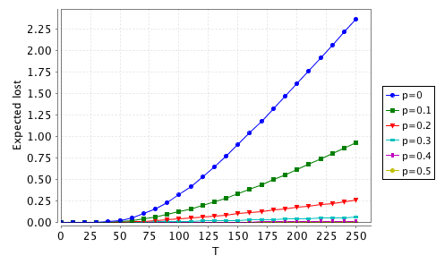
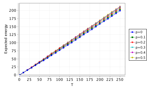
With the new PM component in place,
investigate how the value of p
affects both performance and energy usage, using the two properties above
(i.e., the expected number of lost request and expected energy usage
over the time period 0 to 250). You should get something like the plots below.
As you might expect, increasing p
increases both performance and energy usage.
Can you design a better PM component that offers an improved compromise
between performance and energy usage?
We will now move on to use PRISM's functionality for model checking Markov decision processes (MDPs). This will allow us to explore the best and worst possible PM components that can be devised.
First, change the model type at the top of the PRISM file from
dtmc to
mdp.
Then, replace the choose-labelled commands in the PM module
with a nondeterministic choice between several different commands, shown in the box below.
Also, remove the constant p added above.
Intuitively, this means that the power consumption can pick any of the
choose commands at each step.
	[choose] true -> (pm'=0);
	[choose] q<QMAX -> (pm'=1);
	[choose] q<QMAX -> (pm'=2);
	[choose] q<QMAX -> (pm'=3);
	[choose] q<QMAX -> (pm'=4);
We can now re-investigate some of the properties from above, but on the MDP model.
For example, re-plot the best/worst possible (i.e. min/max)
expected number of lost request and expected energy usage,
preferably overlaid onto the graphs for the DTMC models.
You will need to use properties like the ones below.
You will also need to switch PRISM's model checking engine from "Hybrid" to "Sparse"
using the setting in the "Options" dialog (menu "Options | Options").
R{"lost"}min=? [ C<=T ]
R{"lost"}max=? [ C<=T ]
The behaviour of all of the Power Manager components considered above will fall between the "min" and "max" plots generated in this way.
In principle, we could also extract during this analysis strategies from the MDP that represent designs for Power Manager components exhibiting this best-/worst-case behaviour. In fact, PRISM does not current support strategy generation for this kind of property. In part, this is because they would be history-dependent strategies, which can make different choices at each step, depending on the amount of time that has elapsed. This could also make the power managers inconvenient to implement.
The main problem, though, is that these best- or worst-case scenarios are not very helpful since they optimise one criterion (performance or energy consumption) at the expense of the other. We can resolve this by looking at trade-offs between these conflicting criteria.
Use the following multi-objective
model checking query, representing the property
"what is the minimum possible expected energy consumption within time 250,
whilst keeping the expected number of lost requests below K?".
You will need to add a constant K (of type "double").
We pick 250 because it was the upper limit of the time range we considered above.
Try a value of 1.5 for K.
You should get a result of approximately 149.7.
multi(R{"energy"}min=? [ C<=250 ], R{"lost"}<=K [ C<=250 ])
Use an experiment, varying K,
to see how low the expected energy consumption can be for each different bound
on the expected number of lost requests.
A better way to visualise the trade-off more clearly is to use a Pareto query.
This asks PRISM to compute (approximately) the Pareto curve for this pair objectives.
Intuitively, this is the set of pairs of values (of the expected energy and expected number of lost requests)
such that reducing one value any more would necessitate an increase in the other.
Verify the Pareto query below. The result will be a long list of pairs in this case,
but PRISM also plots the curve for you, which helps to visualise it.
multi(R{"energy"}min=? [ C<=250 ], R{"lost"}min=? [ C<=250 ])
As mentioned above, devising power management modules that actually achieve the optimal values computed above
might be difficult in practice. How close can you get? Devise your own power management strategy,
implemented as a PM module in the DTMC models from above,
and investigate how well they perform.
Can you make it configurable for different constraints on performance or energy consumption?
There is more detailed information about the disk-drive case study you have been looking at here.
You can also find many more interesting examples in the tutorial and case studies sections of the website.