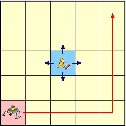
This case study considers an n×n grid world with a robot moving from the bottom left corner to the top right corner, first along the bottom edge and then along the right edge. The time taken by the robot to move from one square to another is exponentially distributed. There is a janitor moving randomly around the grid (initially in the top right hand corner), and the robot cannot move into a square occupied by the janitor. The robot also randomly sends a signal to the base station.

Numerical analysis based on uniformisation and statistical techniques based on sampling and simulation are two distinct approaches for transient analysis of stochastic systems. In this case study we compare the two solution techniques when applied to the verification of time-bounded until formulae in the temporal stochastic logic CSL.
The verification of time-bounded CSL formulae can be reduced to transient analysis [BHHK00a]. Efficient numerical solution techniques, such as uniformisation [Jen53, Gra77], for transient analysis of CTMCs have been existed for decades and are well-understood. Younes and Simmons [YS02] have proposed a statistical approach for verifying time-bounded CSL formulae, based on acceptance sampling and discrete event simulation.
Although the algorithm of Younes and Simmons [YS02] can handle CSL formulae with nested probabilistic operators, the way in which it is done requires in the worst case that the nested formula be verified in each state along a sample path. The numerical approach, on the other hand, can verify the nested formula for all states simultaneously at the same (asymptotic) cost as verifying the formula for a single state. This is a clear advantage when dealing with nested probabilistic operators.
We therefore propose a mixed approach, where statistical sampling is used to verify the outermost probabilistic operator, while numerical techniques are used to verify the nested probabilistic operators. We can mix the numerical and statistical techniques by assuming that the result of the numerical technique holds with certainty. The nested formulae are first verified for all states using numerical methods. When verifying a path formula over a sample path we only need to read the value for each state along the path without any additional verification effort for the nested formulae. The cost for verifying the nested components of a formula is exactly the same for the mixed approach as for the numerical approach, but the use of sampling for the outermost probabilistic operator can provide a solution faster than a numerical computation.
Further details on the comparison between the different methods is available in [YKNP04, YKNP06].
Our PRISM model of the system comprises 2 modules, one for the robot and one for the janitor. Below we give the PRISM language description for the system. Note that to change the size of the grid one need only set the value of the constant n appearing at the start of the description.
// GRID WORLD MODEL OF ROBOT AND JANITOR
// Hakan Younes/gxn/dxp 04/05/04

ctmc

// CONSTANTS
const int n; // size of the grid
const double mr = 1; // rate that the robot moves
const double mj = 2; // rate that the janitor moves
const double cr1 = 1/10; // rate to send a signal to the base station
const double cr2 = 1/2; // rate for communication completion

// the following formulae return 1 or 0 depending on whether
// the janitor can move in that direction or not
formula right = min(1,max(n-x2,0));
formula left = min(1,max(x2-1,0));
formula up = min(1,max(n-y2,0));
formula down = min(1,max(y2-1,0));

// total number of moves the janitor randomly picks from
formula moves = right+left+up+down;

module robot

	x1 : [1..n] init 1; // x position of robot
	y1 : [1..n] init 1; // y position of robot
	c  : [0..1] init 0; // status of signal

	[] x1<n & c=0 & !(x1+1=x2 & y1=y2) -> mr : (x1'=x1+1); // moves right
	[] x1=n & y1<n & c=0 & !(x1=x2 & y1+1=y2) -> mr : (y1'=y1+1); // moves up

	[] c=0 -> cr1 : (c'=1); // send signal
	[] c=1 -> cr2 : (c'=0); // finish communicating

endmodule

module janitor

	x2 : [1..n] init n; // x position of janitor
	y2 : [1..n] init n; // y position of janitor

	[] !(y2=n | (y2+1=y1 & x2=x1)) -> mj/moves : (y2'=y2+1); // moves up
	[] !(y2=1 | (y2-1=y1 & x2=x1))  -> mj/moves : (y2'=y2-1); // moves down
	[] !(x2=1 | (x2-1=x1 & y2=y1))  -> mj/moves : (x2'=x2-1); // moves left
	[] !(x2=n | (x2+1=x1 & y2=y1)) -> mj/moves : (x2'=x2+1); // moves right

endmodule
The tables below shows statistics and construction times of the models when the size of the grid (n) varies. The tables include:
Note that this construction is only required when using the numerical method, as when using the statistical approach, all that we need to store during verification is the current state.
| n: | Model: | MTBDD: | Construction: | ||||||
| States: | Transitions: | Nodes: | Leaves: | Time (s): | Iter.s: | ||||
| 2 | 20 | 53 | 68 | 5 | 0.001 | 6 | |||
| 4 | 216 | 921 | 267 | 5 | 0.01 | 14 | |||
| 8 | 1904 | 9,377 | 627 | 5 | 0.08 | 30 | |||
| 16 | 15840 | 82,737 | 1,326 | 5 | 0.37 | 62 | |||
| 32 | 128960 | 691,793 | 2,749 | 5 | 1.75 | 126 | |||
| 64 | 1.0e+06 | 5.7e+06 | 5,716 | 5 | 8.37 | 254 | |||
| 128 | 8.3e+06 | 4.6e+07 | 11,963 | 5 | 39.18 | 510 | |||
The objective is for the robot to reach the goal square at top right corner within 100 time units with probability at least 0.9, while maintaining at least a 0.5 probability of periodically communicating with the base station. The CSL formula:
expresses the given objective.
In the numerical method we set the truncation error to 1e-6 (stop iterating when the relative error between the iteration vectors is less than 1e-6). On the other hand, when using the statistical approach, the parameters α, β, and δ can be used to trade accuracy for efficiency (see [YS02] for details on these parameters). In the experiments we set α=β=1e-2 and vary δ.
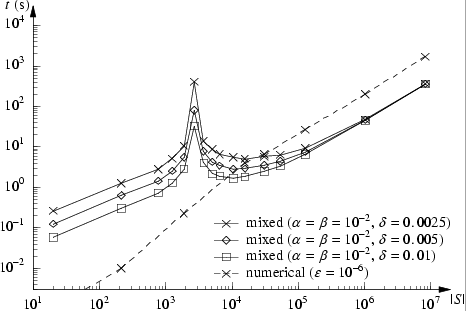
We now report on the results when using the mixed and the numerical approaches. Note that in both methods the inner bounded until (P>=0.5 [ true U<=7 communicate ]) is verified using the numerical approach. The table and graph below compare the overall model checking times of the two approaches (the iterations and samples correspond to those used to verify the outer bounded until).
| n: | Numerial | Statistical | ||||||||
| δ=0.0025 | δ=0.005 | δ=0.01 | ||||||||
| time (s): | iterations: | average time (s): | average no. samples: |
average time (s): | average no. samples: |
average time (s): | average no. samples: |
|||
| 2 | 0.001 | 147 | 0.261 | 828 | 0.124 | 414 | 0.058 | 207 | ||
| 4 | 0.01 | 336 | 1.262 | 828 | 0.626 | 414 | 0.31 | 207 | ||
| 8 | 0.23 | 344 | 10.57 | 2186 | 5.543 | 1141.6 | 2.865 | 582.4 | ||
| 16 | 3.97 | 346 | 5.005 | 474.4 | 2.938 | 246.5 | 1.834 | 120.5 | ||
| 32 | 26.5 | 337 | 9.353 | 270.1 | 7.482 | 133.4 | 6.549 | 63.6 | ||
| 64 | 202.5 | 330 | 47.37 | 144.9 | 45.97 | 71.3 | 45.30 | 34.7 | ||
| 128 | 1677 | 326 | 355.4 | 92 | 354.5 | 46 | 354.2 | 23 | ||
