Cyclic Server Polling System

(Ibe and Trivedi)

Introduction
Model Statistics
Model Construction Times
Model Checking

Introduction:

This case study is based on a cyclic server polling system, taken from [IT90]. The model is represented as a CTMC. We use N to denote the number of stations handled by the polling server. By way of example, the PRISM source code for the case where N=5 is given below.

// polling example [IT90]
// gxn/dxp 26/01/00

ctmc

const int N=5;

const double mu= 1;
const double gamma= 200;
const double lambda= mu/N;

module server

	s : [1..5]; // station
	a : [0..1]; // action: 0=polling, 1=serving
	
	[loop1a] (s=1)&(a=0) -> gamma	: (s'=s+1);
	[loop1b] (s=1)&(a=0) -> gamma	: (a'=1);
	[serve1] (s=1)&(a=1) -> mu	: (s'=s+1)&(a'=0);
	
	[loop2a] (s=2)&(a=0) -> gamma	: (s'=s+1);
	[loop2b] (s=2)&(a=0) -> gamma	: (a'=1);
	[serve2] (s=2)&(a=1) -> mu	: (s'=s+1)&(a'=0);
	
	[loop3a] (s=3)&(a=0) -> gamma	: (s'=s+1);
	[loop3b] (s=3)&(a=0) -> gamma	: (a'=1);
	[serve3] (s=3)&(a=1) -> mu	: (s'=s+1)&(a'=0);
	
	[loop4a] (s=4)&(a=0) -> gamma	: (s'=s+1);
	[loop4b] (s=4)&(a=0) -> gamma	: (a'=1);
	[serve4] (s=4)&(a=1) -> mu	: (s'=s+1)&(a'=0);
	
	[loop5a] (s=5)&(a=0) -> gamma	: (s'=1);
	[loop5b] (s=5)&(a=0) -> gamma	: (a'=1);
	[serve5] (s=5)&(a=1) -> mu	: (s'=1)&(a'=0);
	
endmodule

module station1

	s1 : [0..1];
	
	[loop1a] (s1=0) -> 1 : (s1'=0);
	[]       (s1=0) -> lambda : (s1'=1);
	[loop1b] (s1=1) -> 1 : (s1'=1);
	[serve1] (s1=1) -> 1 : (s1'=0);
	
endmodule

// construct further stations through renaming
module station2 = station1 [s1=s2, loop1a=loop2a, loop1b=loop2b, serve1=serve2] endmodule
module station3 = station1 [s1=s3, loop1a=loop3a, loop1b=loop3b, serve1=serve3] endmodule
module station4 = station1 [s1=s4, loop1a=loop4a, loop1b=loop4b, serve1=serve4] endmodule
module station5 = station1 [s1=s5, loop1a=loop5a, loop1b=loop5b, serve1=serve5] endmodule

// cumulative rewards

rewards "waiting" // expected time the station 1 is waiting to be served
	s1=1 & !(s=1 & a=1) : 1;
endrewards

rewards "served" // expected number of times station1 is served
	[serve1] true : 1;
endrewards

View: printable version Download: polling5.sm

Model Statistics:

The table below shows statistics for each model we have built. The first section gives information about the CTMC representing the model: the number of states and the number of non-zeros (transitions). The second part refers to the MTBDD which represents this CTMC: the total number of nodes, the number of leaves (terminal nodes), and the amount of memory needed to store it. The last column gives the amount of memory a sparse matrix would need to represent the same CTMC.

N:	Model:		MTBDD:			Sparse:
N:	States:	NNZ:	Nodes:	Leaves:	Kb:	Kb:
4	96	272	178	4	3.48	4.3
5	240	800	271	4	5.29	12.2
6	576	2,208	367	4	7.17	32.6
7	1,344	5,824	482	4	14.9	84
8	3,072	14,848	608	4	11.9	210
9	6,912	36,864	765	4	14.9	513
10	15,360	89,600	921	4	18.0	1,230
11	33,792	214,016	1,096	4	21.4	2,904
12	73,728	503,808	1,282	4	25.0	6,768
13	159,744	1,171,456	1,491	4	33.3	15,600
14	344,064	2,695,168	1,707	4	33.3	35,616
15	737,280	6,144,000	1,942	4	37.9	80,640
16	1,572,864	13,893,632	2,188	4	42.7	371,712
17	3,342,336	31,195,136	2,469	4	48.2	378,624
18	7,077,888	69,599,232	2,745	4	53.6	843,264
19	14,942,208	154,402,816	3,040	4	59.4	1,867,776
20	31,457,280	340,787,200	3,346	4	65.4	4,116,362

Model Construction Times

The table below gives the times taken to construct the models. This process involves first building a CTMC (represented as an MTBDD) from the system description (in our module based language), and then computing the reachable states using a BDD based fixpoint algorithm. The total time required and the number of fixpoint iterations are given below.

N:	Construction:
N:	Time (s):	Iter.s:
4	0.039	9
5	0.043	11
6	0.059	13
7	0.063	15
8	0.069	17
9	0.09	19
10	0.107	21
11	0.115	23
12	0.126	25
13	0.144	27
14	0.156	29
15	0.19	31
16	0.202	33
17	0.239	35
18	0.271	37
19	0.302	39
20	0.346	41

Model Checking

We now report on the model checking results obtained using PRISM when checking the following CSL specifications.

// Time bound
const double T;

// Probability that in the long run station 1 is awaiting service 
S=? [ s1=1 & !(s=1 & a=1) ]

// Probability that in the long run station 1 is idle 
S=? [ s1=0 ] 

// Once a station becomes full, the minimum probability it will eventually be polled
P=? [ true U (s=1 & a=0) {s1=1}{min} ]

// Probability, from the inital state, that station 1 is served before station 2
P=? [ !(s=2 & a=1) U (s=1 & a=1) ]

// Probability that station 1 will be polled within T time units
P=?[ true U<=T (s=1 & a=0) ]

// Expected time that station 1 is waiting to be served
R{"waiting"}=?[C<=T]

// Expected number of times station1 is served
R{"served"}=?[C<=T] // number of times station1 is served

View: printable version Download: polling.csl

All experiments were carried out on a 2.80GHz PC with 1 Gb memory running Linux and in all iterative methods we stop iterating when the relative error between subsequent iteration vectors is less than 1e-6, that is:

Computing Steady State Probabilities: the table below gives the model checking statistics when computing these probabilities for both the Jacobi and Gauss-Seidel methods when using PRISM's different engines.

N:	Jacobi:				Gauss Seidel:
	Iters:	Time per iter: (s)			Iters:	Time per iter: (s)
	Iters:	MTBDD	Sparse	Hybrid	Iters:	Sparse	Hybrid
4	130	0.001100	< 0.00001	0.000015	18	< 0.00001	< 0.00001
5	173	0.002931	0.000012	0.000012	20	< 0.00001	< 0.00001
6	218	0.007445	0.000014	0.000028	22	< 0.00001	< 0.00001
7	264	0.020572	0.000042	0.000068	23	0.000087	0.000087
8	310	0.059178	0.000100	0.000158	25	0.000160	0.000320
9	358	0.256704	0.000257	0.000377	26	0.000462	0.000692
10	406	-	0.000643	0.000958	27	0.001037	0.001667
11	455	-	0.001545	0.002455	28	0.002393	0.003893
12	505	-	0.003612	0.006646	29	0.005207	0.009069
13	555	-	0.008295	0.015944	30	0.011733	0.020300
14	606	-	0.019363	0.035465	31	0.026161	0.045065
15	657	-	0.044633	0.080626	32	0.058656	0.104188
16	709	-	0.106413	0.191898	33	0.130212	0.231152
17	761	-	0.235858	0.409599	34	0.288147	0.537794
18	814	-	0.567683	0.908693	34	0.643882	1.187500
19	866	-	1.325487	2.003745	35	1.462714	2.633857
20	920	-	-	4.664724	36	-	5.759333

Probability that in the long run station 1 is awaiting service:
Probability that in the long run station 1 is idle:

Once station 1 becomes full, the minimum probability it will eventually be polled: the table below presents statistics for the model checking process. Note that as this property holds with probability 1 the statistics correspond to a BDD precomputation algorithm.

N:	Iters:	Time per iter: (s)	Minimum probability:
4	18	<0.000001	1
5	22	<0.000001	1
6	26	0.000385	1
7	30	0.000333	1
8	34	0.000294	1
9	38	0.000526	1
10	42	0.000714	1
11	46	0.000870	1
12	50	0.000800	1
13	54	0.001111	1
14	58	0.001207	1
15	62	0.001290	1
16	66	0.001515	1
17	70	0.001714	1
18	74	0.001757	1
19	78	0.002073	1
20	82	0.002308	1

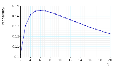
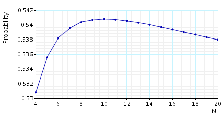
The probability that, from the initial state, station 1 is polled before station 2: the table and below gives the model checking statistics when computing these probabilities for both the Jacobi and Gauss-Seidel methods when using PRISM's different engines.

N:	Jacobi:				Gauss Seidel:
	Iters:	Time per iter: (s)			Iters:	Time per iter: (s)
	Iters:	MTBDD	Sparse	Hybrid	Iters:	Sparse	Hybrid
4	2,480	0.000463	0.000002	0.000002	1,862	0.000009	0.000011
5	2,664	0.000848	0.000005	0.000006	2,285	0.000021	0.000024
6	2,965	0.002041	0.000013	0.000016	2,479	0.000044	0.000045
7	3,124	0.005206	0.000030	0.000041	2,809	0.000095	0.000102
8	3,374	0.013286	0.000076	0.000101	2,965	0.000209	0.000233
9	3,516	0.033981	0.000180	0.000232	3,239	0.000455	0.000516
10	3,732	0.082460	0.000457	0.000560	3,374	0.000993	0.000956
11	3,863	0.193670	0.001076	0.001510	3,612	0.002220	0.002256
12	4,054	0.450005	0.002393	0.004357	3,734	0.004809	0.005239
13	4,176	1.047451	0.005484	0.009719	3,945	0.010381	0.009450
14	4,351	-	0.012999	0.022378	4,058	0.023012	0.021251
15	4,464	-	0.027970	0.049814	4,249	0.049110	0.047892
16	4,623	-	0.066075	0.111454	4,354	0.106876	0.106191
17	4,732	-	0.144911	0.247469	4,529	0.233834	0.243856
18	4,880	-	0.332425	0.554729	4,629	0.539982	0.535855
19	4,983	-	0.769429	1.226136	4,791	1.262000	1.185987
20	5,122	-	-	2.666418	4,886	-	2.657864

The graph below we have plotted these probabilities as the number of stations varies.

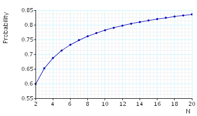
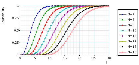
plot: probability that station 1 is served before station 2

The minimum probability that once station 1 is full it is polled within T time units: the table below presents statistics for the model checking process.

N:	T=5:				T=50:
	Iters:	Time per iter: (s)			Iters:	Time per iter: (s)
	Iters:	MTBDD	Sparse	Hybrid	Iters:	MTBDD	Sparse	Hybrid
4	1,299	0.000108	0.000002	0.000004	3,029	0.000097	0.000002	0.000004
5	1,299	0.000360	0.000008	0.000012	3,390	0.000325	0.000006	0.000012
6	1,299	0.000833	0.000017	0.000033	3,735	0.000638	0.000016	0.000032
7	1,299	0.001525	0.000044	0.000089	4,068	0.001276	0.000040	0.000087
8	1,299	0.002905	0.000105	0.000226	4,393	0.002599	0.000100	0.000220
9	1,299	0.005907	0.000259	0.000557	4,709	0.005640	0.000245	0.000545
10	1,299	0.013120	0.000669	0.001400	5,019	0.012821	0.000612	0.001356
11	1,299	0.031202	0.001577	0.003540	5,324	0.030340	0.001483	0.003444
12	1,299	0.073051	0.003677	0.009074	5,625	0.069625	0.003399	0.008809
13	1,299	0.175253	0.008447	0.021134	5,921	0.151677	0.007790	0.020601
14	1,299	0.447443	0.019534	0.048891	6,213	0.350896	0.018084	0.049279
15	1,299	1.332977	0.045169	0.111782	6,503	0.882448	0.041978	0.109156
16	1,299	4.823504	0.109159	0.255657	6,789	2.453282	0.101669	0.249149
17	1,299	-	0.236249	0.574657	7,073	-	0.220543	0.559372
18	1,299	-	0.572048	1.288513	7,355	-	0.538752	1.253214
19	1,299	-	1.376863	2.853521	7,634	-	1.248819	2.778883
20	1,299	-	-	6.311027	7,911	-	-	6.146424

In the graph below, we plot results of the above property for different numbers of stations (values of N):

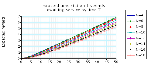
plot: minimum probability that once station 1 is full it is polled within T time units

Expected time station 1 spends awaiting service by time T: the table and graph below we present the model checking statistics as both the number of stations and time bound T varies.

N:	T=5:				T=50:
	Iters:	Time per iter: (s)			Iters:	Time per iter: (s)
	Iters:	MTBDD	Sparse	Hybrid	Iters:	MTBDD	Sparse	Hybrid
4	1,299	0.000270	0.000003	0.000006	3,856	0.000266	0.000004	0.000006
5	1,299	0.000653	0.000008	0.000017	4,766	0.000656	0.000009	0.000017
6	1,299	0.001532	0.000022	0.000040	5,677	0.001534	0.000025	0.000044
7	1,299	0.003857	0.000059	0.000107	6,585	0.003828	0.000063	0.000112
8	1,299	0.010498	0.000142	0.000266	7,489	0.010605	0.000150	0.000276
9	1,299	0.027769	0.000342	0.000649	8,391	0.028500	0.000361	0.000676
10	1,299	0.070794	0.000841	0.001601	9,290	0.075488	0.000865	0.001653
11	1,299	0.175307	0.001948	0.004038	10,187	0.207029	0.002015	0.004120
12	1,299	0.473611	0.004470	0.010046	11,082	0.951248	0.009620	0.010143
13	1,299	1.264613	0.010242	0.023289	11,111	3.642436	0.010285	0.023461
14	1,299	-	0.023290	0.053094	11,111	-	0.023422	0.053808
15	1,299	-	0.052793	0.120839	11,112	-	0.053346	0.121939
16	1,299	-	0.124015	0.273636	11,112	-	0.126152	0.276256
17	1,299	-	0.269986	0.611949	11,112	-	0.274005	0.616791
18	1,299	-	0.639747	1.400105	11,112	-	0.650463	1.371019
19	1,299	-	-	3.016768	11,112	-	-	3.030094
20	1,299	-	-	6.629515	11,112	-	-	6.676664

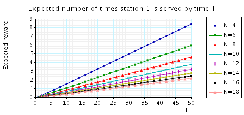
plots expected time station 1 spends awaiting service by time T

Expected number of times station 1 is served by time T:

Cyclic Server Polling System

Contents

Introduction:

Model Statistics:

Model Construction Times

Model Checking

Case Studies