
(Lynch, Saias and Segala)
This case study is based on Lehmann and Rabin's solution to the well known dining philosophers problem [LR81] and the analysis of this algorithm by Lynch, Saias and Segala [LSS94]. In particular, Lynch, Saias and Segala consider proving time bounds for this algorithm by making the following assumption:
Under this assumption, Lynch, Saias and Segala proved that the following property holds:
However, since we only model discrete time we cannot make the assumption given above. Instead we make the following assumption:
This is a stronger assumption than that of Lynch, Saias and Segala, and hence we consider a smaller class of adversaries or schedulers. As a result, we can prove stronger properties than that given above (dependent on the value of K).
The model is represented as an MDP. In the following, N denotes the number of philosophers and K is as above, i.e. the maximum number of transitions that can occur between a philosopher in its trying region being scheduled. By way of example, the PRISM source code for the case where N=3 is given below.
// Lehmann-Rabin algorithm [LR82] (dining philosophers)
// we suppose an action takes 1 time unit
// an a process can wait at most K time units before making a transition
// gxn/dxp 01/02/00

mdp

// CONSTANTS
const K;

// COUNTER FORMULAE
// ci number of steps since process last moved
// removing trying and remainder states since
// these are controlled by the process not the adversary

// process can go if it does not stop one of the other processes round counter reaching K+1
// added complication if two processes counter equals K-1, then if neither makes a transition
// both reach K, and hence one must reach K+1 which we must disallow
formula can1 = !((c2=K) | (c3=K) | ((c2=K-1) & (c3=K-1)));
formula can2 = !((c1=K) | (c3=K) | ((c1=K-1) & (c3=K-1)));
formula can3 = !((c1=K) | (c2=K) | ((c1=K-1) & (c2=K-1)));

// when a process moves the counters of the other processes increase
// but only when they are not in trying or remainder
formula count1  = (p1!=13) & (p1!=0);
formula count2  = (p2!=13) & (p2!=0);
formula count3  = (p3!=13) & (p3!=0);
formula ncount1 = (p1=13) | (p1=0);
formula ncount2 = (p2=13) | (p2=0);
formula ncount3 = (p3=13) | (p3=0);

module counter

	c1 : [0..K];
	c2 : [0..K];
	c3 : [0..K];

	// process 1 moves
	[s1] count2  & count3  & can1 -> (c1'=0) & (c2'=c2+1) & (c3'=c3+1);
	[s1] ncount2 & count3  & can1 -> (c1'=0) & (c3'=c3+1);
	[s1] count2  & ncount3 & can1 -> (c1'=0) & (c2'=c2+1);
	[s1] ncount2 & ncount3 & can1 -> (c1'=0);
	// process 2 moves
	[s2] count1  & count3  & can2 -> (c2'=0) & (c1'=c1+1) & (c3'=c3+1);
	[s2] ncount1 & count3  & can2 -> (c2'=0) & (c3'=c3+1);
	[s2] count1  & ncount3 & can2 -> (c2'=0) & (c1'=c1+1);
	[s2] ncount1 & ncount3 & can2 -> (c2'=0);
	// process 3 moves
	[s3] count1  & count2  & can3 -> (c3'=0) & (c1'=c1+1) & (c2'=c2+1);
	[s3] ncount1 & count2  & can3 -> (c3'=0) & (c2'=c2+1);
	[s3] count1  & ncount2 & can3 -> (c3'=0) & (c1'=c1+1);
	[s3] ncount1 & ncount2 & can3 -> (c3'=0);

endmodule

// PHILOSOPHER 1
// atomic formule
// left fork and right fork free resp.
formula lfree = p2>=0&p2<=4|p2=6|p2=11|p2=13;
formula rfree = p3>=0&p3<=3|p3=5|p3=7|p3=12|p3=13;

module phil1

	p1 : [0..13];

	[s1] (p1=0) -> (p1'=0); // try
	[s1] (p1=0) -> (p1'=1);
	[s1] (p1=1) -> 0.5 : (p1'=2) + 0.5 : (p1'=3); // flip
	[s1] (p1=2) &  lfree -> (p1'=4); // wl and l free
	[s1] (p1=2) & !lfree -> (p1'=2); // wl and l taken
	[s1] (p1=3) &  rfree -> (p1'=5); // wr and r free
	[s1] (p1=3) & !rfree -> (p1'=3); // wr and r taken
	[s1] (p1=4) &  rfree -> (p1'=8); // l and r free
	[s1] (p1=4) & !rfree -> (p1'=6); // l and r taken
	[s1] (p1=5) &  lfree -> (p1'=8); // r and l free
	[s1] (p1=5) & !lfree -> (p1'=7); // r and l taken
	[s1] (p1=6)  -> (p1'=1); // nr
	[s1] (p1=7)  -> (p1'=1); // nl
	[s1] (p1=8)  -> (p1'=9); // pre_crit
	[s1] (p1=9)  -> (p1'=10); // crit
	[s1] (p1=10) -> (p1'=11); // exit
	[s1] (p1=10) -> (p1'=12);
	[s1] (p1=11) -> (p1'=13); // put down left first
	[s1] (p1=12) -> (p1'=13); // put down right first
	[s1] (p1=13) -> (p1'=0); // remainder
	[s1] (p1=13) -> (p1'=13);

endmodule

// construct further processes through renaming
module phil2=phil1 [p1=p2, p2=p3, p3=p1, s1=s2] endmodule
module phil3=phil1 [p1=p3, p2=p1, p3=p2, s1=s3] endmodule

// reward structure - number of steps
rewards "steps"
	[s1] true : 1;
	[s2] true : 1;
	[s3] true : 1;
endrewards
The table below shows statistics for the MDPs we have built for different values of the constants N and K. The tables include:
| N: | K: | Model: | MTBDD: | Construction: | ||||||
| States: | Transitions: | Nodes: | Leaves: | Time (s): | Iter.s: | |||||
| 3 | 4 | 28,940 | 77,292 | 11,805 | 3 | 1.465 | 27 | |||
| 5 | 47,204 | 135,636 | 15,235 | 3 | 1.630 | 27 | ||||
| 6 | 69,986 | 211,344 | 18,691 | 3 | 2.358 | 28 | ||||
| 7 | 97,298 | 304,152 | 21,063 | 3 | 2.757 | 29 | ||||
| 8 | 129,254 | 414,318 | 25,014 | 3 | 3.649 | 30 | ||||
| 9 | 165,746 | 541,908 | 27,072 | 3 | 3.534 | 31 | ||||
| 10 | 206,864 | 686,820 | 28,506 | 3 | 5.024 | 32 | ||||
| 4 | 4 | 729,080 | 1,876,960 | 76,041 | 3 | 17.87 | 34 | |||
| 5 | 1,692,144 | 5,035,016 | 121,758 | 3 | 32.17 | 42 | ||||
| 6 | 3,269,200 | 10,704,752 | 179,714 | 3 | 50.34 | 36 | ||||
| 7 | 5,609,336 | 19,662,904 | 242,666 | 3 | 75.78 | 37 | ||||
| 8 | 8,865,024 | 32,653,704 | 314,314 | 3 | 57.07 | 38 | ||||
| 9 | 13,192,376 | 50,438,968 | 374,738 | 3 | 98.06 | 39 | ||||
| 10 | 18,740,512 | 73,785,912 | 425,481 | 3 | 102.5 | 40 | ||||
When model checking, we have the following requirements:
These correspond to the conditions on the adversary/scheduler with the first being imposed by model checking against only fair adversaries.
The properties we have model checked are given below.
const int L; // discrete time bound

label "trying" =((p1>0) & (p1<8))  | ((p2>0) & (p2<8)) | ((p3>0) & (p3<8)); // philosopher in its trying region
label "entered" =((p1>7) & (p1<13)) | ((p2>7) & (p2<13)) | ((p3>7) & (p3<13)); // philosopher in its critical section

// lockout free
"trying" =>  P>=1 [ true U "entered" ]

// bounded until: minimum probability (from a state where a process is in its trying region) that some process enters its critical section within k steps
Pmin=? [ true U<=L "entered" {"trying"}{min} ]

// expected time: maximum expected time (from a state where a process is in its trying region) that some process enters its critical section
Rmax=? [ F "entered" {"trying"}{max} ]
Theorem 5 from [LR81] (Lockout Free) the model checking statistics for this property are given below.
| N: | K: | Precomputation: | Main Algorithm: | ||||||
| Prob0E: | Prob1A: | ||||||||
| Time (s): | Iterations: | Time (s): | Iterations: | Time (s): | Iterations: | ||||
| 3 | 4 | 0.64 | 0.64 | 1 | 0.01 | - | - | ||
| 5 | 0.85 | 0.85 | 1 | 0.02 | - | - | |||
| 6 | 1.52 | 1.52 | 1 | 0.02 | - | - | |||
| 7 | 1.96 | 1.96 | 1 | 0.02 | - | - | |||
| 8 | 3.02 | 3.02 | 1 | 0.03 | - | - | |||
| 9 | 3.27 | 3.27 | 1 | 0.03 | - | - | |||
| 10 | 3.76 | 3.76 | 1 | 0.03 | - | - | |||
| 4 | 4 | 6.33 | 23 | 1 | 0.09 | - | - | ||
| 5 | 13.5 | 28 | 1 | 0.14 | - | - | |||
| 6 | 26.4 | 31 | 1 | 0.20 | - | - | |||
| 7 | 45.1 | 34 | 1 | 0.28 | - | - | |||
| 8 | 70.7 | 37 | 1 | 0.35 | - | - | |||
| 9 | 114 | 41 | 1 | 0.40 | - | - | |||
| 10 | 160 | 45 | 1 | 0.58 | - | - | |||
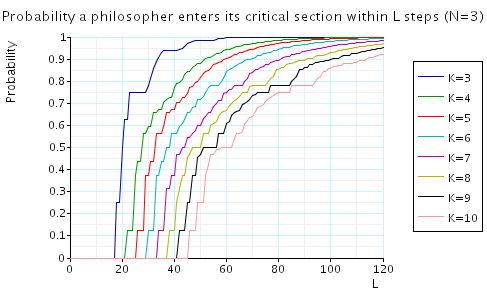
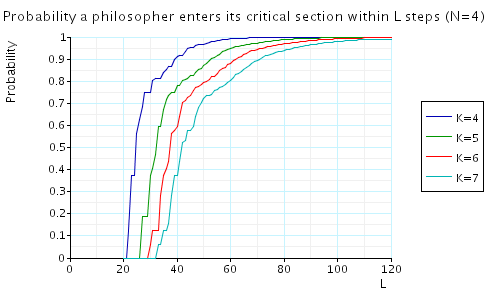
Bounded waiting: in the graphs below we have plotted these expected values as L varies for a range of values of N and K.
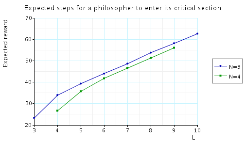
Expected time: in the graph below we have plotted these expected values for a range of values of N and K.