

Related publications: [DKN02, DKN04]
This case study concerns the Tree Identify Protocol of the IEEE 1394 High Performance Serial Bus (called ''FireWire''). The 1394 High Performance serial bus is used to transport video and audio signals within a network of multimedia devices. It has a scalable architecture and is ''hot-pluggable'', meaning that at any time devices can easily be added or removed from the network.
The tree identify process of IEEE 1394 is a leader election protocol which takes place after a bus reset in the network, that is, when a node is added or removed from the network. After such a reset all nodes in the network have equal status, and know only to which nodes they are directly connected. A leader (root) needs to be chosen to act as the manager of the bus for subsequent phases of IEEE 1394. This is done by the nodes communicating ''be my parent'' messages, starting from the leaf nodes. It can happen that two nodes contend the leadership (root contention), in which case the contenders exchange additional messages and involve time delays and electronic coin tosses.
The protocol is designed for use on connected networks, will correctly elect a leader if the network is acyclic, and will report an error if a cycle is detected. For further information concerning the IEEE 1394 Tree Identify Protocol see here.
We consider the following probabilistic timed automata models of the root contention part of the tree identify protocol, which are based on probabilistic I/O automata models presented in [SV99].
We first use timed automata model checking tool KRONOS to perform a symbolic forwards reachability analysis to generate the set of states that are reachable with non-zero probability from the initial state, and before the deadline expires. This information is then encoded as a Markov decision process which we analyse with PRISM. We apply this technique to compute the minimum probability of a leader being elected before a deadline, for different deadlines, and study the influence of using a biased coin on this minimal probability.
Further details are available in [DKN02, DKN04].
The forwards reachability algorithm of KRONOS proceeds by a graph-theoretic traversal of the reachable state space using a symbolic representation of states called symbolic states [DT98]. For example, consider the following probabilistic timed automata.

The above probabilistic timed automata models a process which repeatedly tries to send a packet after between 4 and 5 seconds, and if successful waits for 3 seconds before trying to send another packet. The packet is sent with probability 0.99 and lost with probability 0.01 due to an error.
The reachability graph obtained for the above probabilistic timed automata for a deadline of 15 seconds, measured with an extra clock y is given below. Since4 y is never reset, its value would increase indefinitely. To obtain a finite reachability graph, we need to apply the extrapolation abstraction of [DT98], which abstract away the exact value of y when y>=15. Notice that the abstraction is exact with respect to reachability properties.

The reachability graph obtained with KRONOS is described by an explicit list of states and transitions. In order to model check probabilistic properties we must encode it as a Markov decision process using PRISM's description language.
The behaviour of a system is described by a set of guarded commands of the form:
[] guard -> command.
A guard is a predicate over variables of the system. A command describes a transition which the system can make if the guard is true, by giving a new value to primed variables as a function on the old values of unprimed variables. We consider two types of encoding of a reachability graph in this language.
The first solution is a direct explicit encoding of the reachability graph using a single variable s whose value is the index of the state of the reachability graph. Transitions of the system are encoded by guarded commands such that the guard tests the value of s and the command updates it according to the transition relation of the reachability graph. For example, the encoding of the outgoing transitions from states 0, 4 and 7, corresponding to location send in the reachability graph above is:
	[] s=0 -> 0.99: (s'=1) + 0.01: (s'=2);
	[] s=4 -> 0.99: (s'=5) + 0.01: (s'=6);
	[] s=7 -> 0.99: (s'=8) + 0.01: (s'=9);
This encoding generates a description the size of the reachability graph, which can grow drastically with the value of the deadline. PRISM involves a model construction phase, during which the system description is parsed and converted into an MTBDD representation for further analysis. This phase can be extremely time consuming when the input file does not correspond to a modular and structured description of a system, such as with the explicit encoding. Thus, an encoding allowing for a more compact description of the system is needed. Below we outline a number of compaction techniques and also consider an alternative approach where instead we reduce the size of the reachability graph through applying a probabilistic bisimulation [SL94] quotient.
Symbolic states in the reachability graph correspond to several instances of locations of the timed automaton from which it was generated, with different time constraints. We can then encode them with two variables: a location variable l and an instance variable n describing to which instance of the location it corresponds.
Let l = 0, 1, 2 and 3 be the values corresponding to locations send, wait, error, and error_before respectively. Then, symbolic states 0, 4 and 7 correspond to three different instances of location send, say n = 0, 1 and 2. The outgoing probabilistic transitions from these states can be specified by the guarded commands:
	[] l=0 & n=0 -> 0.99 : (l'=1) & (n'=0) + 0.01 : (l'=2) & (n'=0);
	[] l=0 & n=1 -> 0.99 : (l'=1) & (n'=1) + 0.01 : (l'=2) & (n'=1);
	[] l=0 & n=2 -> 0.99 : (l'=1) & (n'=2) + 0.01 : (l'=2) & (n'=2);
Similarly, symbolic state 3 is the unique instance of location error_before, encoded as l=3 and n=0. The incoming transitions to this state are described by:
	[] l=2 & n=0 -> 1 : (l'=3) & (n'=0);
	[] l=2 & n=1 -> 1 : (l'=3) & (n'=0);
Instances are computed by a breadth-first traversal of the reachability graph.
Note that, in the commands representing the outgoing transitions from location send, the instance variable n is left unchanged, meaning that the transition only affects the location variable for instances 0, 1 and 2. This is equivalent to write that n'=n, which can be omitted since, by default, a non updated variable takes its old value. Thus, the transitions above have the same update command, and can then be described more compactly in a single command line:
[] l=0 & (n=0 | n=1 | n=2) -> 0.99 : (l'=1) + 0.01 : (l'=2);
In a reachability graph, a transition between two given locations is usually repeated several times for different instances of the locations. This encoding allows us to specify them all in a single command line.
We will refer to this as the relative compaction, because it is based on specifying the updated value n' relative to its old value n.
The previous compaction does not apply in the case of the two incoming transitions to error_before. However, if we specify the updated value n' with its absolute value, the update command of both transitions is the same. Thus, they can both be described more compactly in a single command line:
[] l=2 & (n=0 | n=1) -> 1 : (l'=3) & (n'=0);
In a reachability graph, we encounter states which are the destination of many different transitions, such as the state encoded by l=3 and n=0. This encoding allows us to specify them all in a single command line.
We will refer to this as the absolute compaction, because it is based on specifying the absolute value of n'. Note that this compaction could also be applied to the explicit encoding. However, since in practice the relative compaction leads to a more compact description, compaction algorithms have only been implemented in the case of the instances encoding. Absolute compaction is especially interesting when used in combination with the relative one.
In order to obtain a further reduction, we can combine both compactions. Since in practice there are potentially more transitions to be compacted with the relative encoding than with the absolute one, the heuristic implemented consists in first applying the relative compaction and then, for those transitions that were not compacted, i.e. those whose guard correspond to a unique source state, to change the command updates for the instance variable n from relative to absolute, and then apply the absolute compaction.
As an alternative approach we use the CADP (Ceasar/Aldebaran Development Package) a tool set for the design and verification of complex systems, which has recently be extended to allow for performance evaluation [GH02]. In particular, we use the bcg_min tool which supports the minimisation of probabilistic systems with respect to probabilistic bisimulation. The main steps in this approach are: represent the reachability graph in a format suitable for the CADP toolset, use CADP to construct the bisimulation quotient, and finally translate the CADP output into the PRISM language.
To construct the input to CADP required only a straightforward modification of the output from KRONOS (the main step is converting the reachability graph to the alternating model [HJ94]). For the quotient system to preserve the maximal reachability probability of interest, we must identify the states where a leader has been elected after the deadline has passed. For simplicity, since these are the only states that we need to identify, we add loops to these states and label these transition with one action and then label all remaining transitions with another distinct action.
Using this version of the reachability graph, we then use the toolset CADP to construct the quotient under probabilistic bisimulation which preserves the maximal probability of electing a leader after the deadline has passed.
To translate the CADP output into the PRISM language we wrote a simple translator which takes as input the probabilistic system representing the quotient system (the output from CADP) and translates this into the PRISM language. We note that at this stage we have lost all information concerning which locations and zones correspond to which states, and hence we are restricted to an explicit encoding of the quotient system.
In the case when DEADLINE=4,000, the KRONOS source code can be found here and the output files when using the different encodings and compaction algorithms are listed below.
Also in the case when DEADLINE=4,000, the input and output files from CADP can be found here and here respectively.
In the table below we summarise the results concerning the generation with KRONOS of the reachability graph and of its encoding as an MDP in PRISM's description language.
| DEADLINE (103ns): | forward reachability: | reduced model: | encoding in PRISM language (lines): | ||||||||
| explicit: | instances: | ||||||||||
| states: | time (sec): | states: | unreduced: | reduced | absolute | relative | relative+absolute | ||||
| 4 | 2599 | 0.940 | 104 | 3716 | 124 | 2424 | 974 | 894 | |||
| 6 | 4337 | 1.64 | 182 | 6202 | 219 | 4050 | 1545 | 1473 | |||
| 8 | 7831 | 2.93 | 285 | 11262 | 344 | 7320 | 2748 | 2622 | |||
| 10 | 11119 | 4.27 | 486 | 15986 | 588 | 10398 | 3864 | 3710 | |||
| 20 | 41017 | 18.7 | 1639 | 59254 | 1988 | 38406 | 14062 | 13730 | |||
| 30 | 89283 | 56.1 | 3576 | 129154 | 4340 | 83634 | 30349 | 29843 | |||
| 40 | 155675 | 129 | 6147 | 225420 | 7462 | 145854 | 52681 | 52019 | |||
| 50 | 241125 | 225 | 9484 | - | 11514 | - | - | - | |||
| 60 | 344719 | 441 | 13501 | - | 16392 | - | - | - | |||
| 80 | 607871 | 1312 | 23146 | - | 28104 | - | - | - | |||
Furthermore, the graph below shows the evolution of the number of lines of the generated file for the different values of the deadline. It demonstrates that the instances encoding allows for compactions which reduce drastically the number of lines of the MDP file, but quotienting by probabilistic bisimulation achieves the greatest reduction.

In the case when DEADLINE=10,000, the KRONOS source code can be found here and the output files when using the different encodings and compaction algorithms are listed below.
Also in the case when DEADLINE=10,000, the input and output files from CADP can be found here and here respectively.
In the table below we summarise the results concerning the generation with KRONOS of the reachability graph and of its encoding as an MDP in PRISM's description language.
| DEADLINE (103ns): | forward reachability: | reduced model: | encoding in PRISM language (lines): | ||||||||
| explicit: | instances: | ||||||||||
| states: | time (sec): | states: | unreduced: | reduced | absolute | relative | relative+absolute | ||||
| 4 | 131 | 0.00 | 32 | 174 | 39 | 104 | 42 | 26 | |||
| 6 | 216 | 0.01 | 67 | 290 | 83 | 173 | 64 | 27 | |||
| 8 | 372 | 0.02 | 83 | 499 | 103 | 297 | 91 | 36 | |||
| 10 | 526 | 0.03 | 111 | 709 | 138 | 421 | 126 | 39 | |||
| 20 | 1,876 | 0.09 | 454 | 2531 | 566 | 1501 | 368 | 72 | |||
| 30 | 4,049 | 0.20 | 976 | 5466 | 1219 | 3240 | 734 | 100 | |||
| 40 | 7,034 | 0.46 | 1764 | 9499 | 2205 | 5629 | 1223 | 126 | |||
| 50 | 10,865 | 1.23 | 2732 | 14674 | 3417 | 8694 | 1842 | 159 | |||
| 60 | 15,511 | 2.74 | 3854 | 20952 | 4821 | 12412 | 2586 | 186 | |||
| 80 | 27,296 | 8.94 | 6608 | 36868 | 8267 | 21841 | 4437 | 243 | |||
| 100 | 42,401 | 22.2 | 10268 | 57274 | 12841 | 33926 | 6797 | 303 | |||
Furthermore, the graph below shows the evolution of the number of lines of the generated file for the different values of the deadline. It demonstrates that the instances encoding allows for compactions which reduce drastically the number of lines of the MDP file, and in the case where both relative and absolute compactions are used, the number of lines grows less than linearly on the value of the deadline and offers a greater reduction than applying the probabilistic bisimulation quotient.

We now report on the model checking results when using PRISM for both Impl and Abst models. We first compute the minimum probability of a leader being elected before a deadline, for different deadlines, and then study the influence of using a biased coin on this minimal probability.
The table below shows statistics for the MTBDD which represents each model we have built, in terms of the the total number of nodes and the number of leaves (terminal nodes), for each of the encodings and compaction algorithms.
| Impl Model | ||||||||||||
| DEADLINE (103ns): | Nodes: | Leaves: | ||||||||||
| explicit: | instances: | |||||||||||
| unreduced: | reduced | absolute | relative | relative+absolute | ||||||||
| 4 | 5,217 | 411 | 2,017 | 1,787 | 1,791 | 3 | ||||||
| 6 | 7,582 | 727 | 2,592 | 2,165 | 2,259 | 3 | ||||||
| 8 | 11,736 | 1,117 | 3,648 | 2,917 | 2,937 | 3 | ||||||
| 10 | 15,202 | 1,821 | 4,576 | 3,579 | 3,609 | 3 | ||||||
| 20 | - | 4,900 | 9,464 | 6,799 | 6,853 | 3 | ||||||
| 30 | - | 9,624 | - | 9,720 | 9,785 | 3 | ||||||
| 40 | - | 15,520 | - | 12,358 | 12,437 | 3 | ||||||
| 50 | - | 18,130 | - | - | - | 3 | ||||||
| 60 | - | 29,118 | - | - | - | 3 | ||||||
| 80 | - | 45,537 | - | - | - | 3 | ||||||
| Abst Model | ||||||||||||
| DEADLINE (103ns): | Nodes: | Leaves: | ||||||||||
| explicit: | instances: | |||||||||||
| unreduced: | reduced | absolute | relative | relative+absolute | ||||||||
| 4 | 485 | 140 | 188 | 188 | 193 | 3 | ||||||
| 6 | 698 | 341 | 346 | 328 | 328 | 3 | ||||||
| 8 | 979 | 375 | 403 | 403 | 405 | 3 | ||||||
| 10 | 1,306 | 468 | 488 | 473 | 473 | 3 | ||||||
| 20 | 2,676 | 1,506 | 988 | 971 | 991 | 3 | ||||||
| 30 | 4,422 | 2,874 | 1,662 | 1,515 | 1,548 | 3 | ||||||
| 40 | - | 4,502 | 2,214 | 2,007 | 2,053 | 3 | ||||||
| 50 | - | 6,267 | 2,581 | 2,311 | 2,390 | 3 | ||||||
| 60 | - | 7,762 | 3,387 | 3,056 | 3,165 | 3 | ||||||
| 80 | - | 11,121 | 4,396 | 3,855 | 4,007 | 3 | ||||||
| 100 | - | 15,114 | - | 5,293 | 5,451 | 3 | ||||||
The tables below gives the times taken to construct the models.
| Impl Model | ||||||||
| DEADLINE: | Construction time (s): | |||||||
| explicit: | instances: | |||||||
| unreduced: | reduced | relative | absolute | relative+absolute | ||||
| 4 | 270 | 0.268 | 8.37 | 5.67 | 4.86 | |||
| 6 | 878 | 0.711 | 19.2 | 13.4 | 10.9 | |||
| 8 | 2,640 | 1.85 | 61.9 | 44.8 | 38.1 | |||
| 10 | 6,078 | 5.08 | 129 | 96.5 | 82.1 | |||
| 20 | - | 81.8 | 2,099 | 1,719 | 1,469 | |||
| 30 | - | 389 | - | 9,057 | 7,614 | |||
| 40 | - | 1,305 | - | 30,977 | 27,870 | |||
| 50 | - | 3,451 | - | - | - | |||
| 60 | - | 7,172 | - | - | - | |||
| 80 | - | 23,320 | - | - | - | |||
| Abst Model | ||||||||
| DEADLINE: | Construction time (s): | |||||||
| explicit: | instances: | |||||||
| unreduced: | reduced | absolute | relative | relative+absolute | ||||
| 4 | 0.492 | 0.092 | 0.124 | 0.101 | 0.056 | |||
| 6 | 1.14 | 0.167 | 0.202 | 0.155 | 0.071 | |||
| 8 | 3.79 | 0.208 | 0.390 | 0.067 | 0.105 | |||
| 10 | 8.54 | 0.339 | 0.645 | 0.245 | 0.136 | |||
| 20 | 122 | 5.79 | 6.29 | 1.82 | 0.505 | |||
| 30 | 698 | 27.6 | 33.2 | 8.97 | 1.50 | |||
| 40 | - | 111 | 112 | 26.8 | 3.70 | |||
| 50 | - | 284 | 289 | 71.1 | 8.21 | |||
| 60 | - | 554 | 612 | 147 | 15.4 | |||
| 80 | - | 1,802 | 2,187 | 531 | 43.1 | |||
| 100 | - | 5,181 | - | 1,486 | 91.9 | |||
The property we consider is: "the minimum probability that a leader (root) is chosen before a DEADLINE."
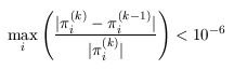
Using a fair coin: In the table below, summarises the model checking results when using a fair coin and both the most compact encoding (instances encoding with both the absolute and relative compaction algorithms) and the explicit encoding and the reduced reachability graph, when using the MTBDD, sparse and hybrid engines, where in each case we stop iterating when the relative error between subsequent iteration vectors is less than 1e-6, that is:
Model checking times:
| Impl Model | ||||||||||||||||
| DEADLINE: | unreduced: instances rel+abs | reduced: explicit | Probability: | |||||||||||||
| Time per iteration (s): | Iterations: | Time per iteration (s): | Iterations: | |||||||||||||
| MTBDD | Sparse | Hybrid | MTBDD | Sparse | Hybrid | |||||||||||
| 4 | 0.00090 | < 0.00001 | < 0.00001 | 11 | < 0.00001 | < 0.00001 | < 0.00001 | 15 | 0.625000000 | |||||||
| 6 | 0.00185 | < 0.00001 | 0.00037 | 27 | 0.00057 | < 0.00001 | < 0.00001 | 35 | 0.851562500 | |||||||
| 8 | 0.00457 | < 0.00001 | 0.00029 | 35 | 0.00111 | < 0.00001 | < 0.00001 | 45 | 0.939453135 | |||||||
| 10 | 0.00725 | 0.00039 | 0.00078 | 51 | 0.00215 | < 0.00001 | < 0.00001 | 65 | 0.974731455 | |||||||
| 20 | 0.06609 | 0.00235 | 0.00469 | 115 | 0.01496 | 0.00006 | 0.00034 | 145 | 0.999629565 | |||||||
| 30 | 0.29515 | 0.00544 | 0.01128 | 171 | 0.07934 | 0.00014 | 0.00079 | 215 | 0.999994454 | |||||||
| 40 | 0.67436 | 0.01132 | 0.02118 | 227 | 0.21943 | 0.00021 | 0.00171 | 285 | 0.999999919 | |||||||
| 50 | - | - | - | - | 0.37234 | 0.00031 | 0.00235 | 353 | 0.999999998 | |||||||
| 60 | - | - | - | - | 0.83342 | 0.00045 | 0.00390 | 415 | 0.999999999 | |||||||
| 80 | - | - | - | - | 2.23935 | 0.00095 | 0.00640 | 545 | 1.000000000 | |||||||
| Abst Model | ||||||||||||||||
| DEADLINE: | unreduced: instances rel+abs | reduced: explicit | Probability: | |||||||||||||
| Time per iteration (s): | Iterations: | Time per iteration (s): | Iterations: | |||||||||||||
| MTBDD | Sparse | Hybrid | MTBDD | Sparse | Hybrid | |||||||||||
| 4 | < 0.00001 | < 0.00001 | < 0.00001 | 6 | < 0.00001 | < 0.00001 | < 0.00001 | 8 | 0.625000000 | |||||||
| 6 | < 0.00001 | < 0.00001 | < 0.00001 | 12 | < 0.00001 | < 0.00001 | < 0.00001 | 16 | 0.851562500 | |||||||
| 8 | < 0.00001 | < 0.00001 | < 0.00001 | 15 | < 0.00001 | < 0.00001 | < 0.00001 | 20 | 0.939453135 | |||||||
| 10 | 0.00048 | < 0.00001 | < 0.00001 | 21 | 0.00036 | < 0.00001 | < 0.00001 | 28 | 0.974731455 | |||||||
| 20 | 0.00089 | < 0.00001 | 0.00022 | 45 | 0.00233 | < 0.00001 | < 0.00001 | 60 | 0.999629565 | |||||||
| 30 | 0.00151 | 0.00015 | 0.00030 | 66 | 0.01022 | 0.00022 | < 0.00001 | 88 | 0.999994454 | |||||||
| 40 | 0.00218 | 0.00046 | 0.00058 | 87 | 0.02491 | 0.00035 | 0.00008 | 116 | 0.999999919 | |||||||
| 50 | 0.00428 | 0.00037 | 0.00084 | 107 | 0.05886 | 0.00049 | 0.00007 | 142 | 0.999999998 | |||||||
| 60 | 0.01131 | 0.00064 | 0.00151 | 126 | 0.09722 | 0.00071 | 0.00011 | 168 | 0.999999999 | |||||||
| 80 | 0.00793 | 0.00133 | 0.00290 | 165 | 0.22117 | 0.00146 | 0.00018 | 220 | 1.000000000 | |||||||
| 100 | 0.01374 | 0.00211 | 0.00456 | 204 | 0.06867 | 0.00365 | 0.00253 | 260 | 1.000000000 | |||||||
Varying the communication delay between the nodes: In the figure below, we give the probability for electing a leader before a deadline as the communication delay (wire length) between the nodes varies. As expected the results show that the probability of electing a leader before a deadline decreases as the communication delay decreases.

Varying the coin bias: In the tables below, we give the probability for electing a leader before a deadline of 3,000ns, 4,0000ns, 6,000ns, 8,0000ns and 10,000ns, for different biased coins (different probabilities of choosing the fast and slow timings) when the communication delay is both 360ns and 30ns.
| fast: | slow: | communication delay 30ns | communication delay 360ns | ||||||||||
| 3,000ns: | 4,000ns: | 6,000ns: | 8,000ns: | 10,000ns: | 3,000ns: | 4,000ns: | 6,000ns: | 8,000ns: | 10,000ns: | ||||
| 0.01 | 0.99 | 0.019802 | 0.039208 | 0.058237 | 0.076886 | 0.095166 | 0.019800 | 0.019803 | 0.039211 | 0.058237 | 0.076886 | ||
| 0.10 | 0.90 | 0.181800 | 0.327618 | 0.452219 | 0.551777 | 0.633233 | 0.180000 | 0.181800 | 0.330534 | 0.452219 | 0.551770 | ||
| 0.20 | 0.80 | 0.332800 | 0.538112 | 0.702301 | 0.801006 | 0.866886 | 0.320000 | 0.332800 | 0.554516 | 0.702353 | 0.801000 | ||
| 0.30 | 0.70 | 0.457800 | 0.667002 | 0.837450 | 0.910965 | 0.950908 | 0.420000 | 0.457800 | 0.704352 | 0.838050 | 0.910950 | ||
| 0.40 | 0.60 | 0.556800 | 0.741888 | 0.904804 | 0.957200 | 0.980052 | 0.480000 | 0.556800 | 0.799150 | 0.907635 | 0.957090 | ||
| 0.45 | 0.55 | 0.595238 | 0.765273 | 0.922093 | 0.968547 | 0.986339 | 0.495000 | 0.595238 | 0.830027 | 0.927066 | 0.968230 | ||
| 0.50 | 0.50 | 0.625000 | 0.781250 | 0.931641 | 0.975494 | 0.989969 | 0.500000 | 0.625000 | 0.851562 | 0.939453 | 0.974731 | ||
| 0.51 | 0.49 | 0.629797 | 0.783612 | 0.932769 | 0.976489 | 0.990474 | 0.499800 | 0.629797 | 0.854832 | 0.941215 | 0.975592 | ||
| 0.52 | 0.48 | 0.634183 | 0.785698 | 0.933662 | 0.977373 | 0.990919 | 0.499200 | 0.634183 | 0.857768 | 0.942757 | 0.976322 | ||
| 0.53 | 0.47 | 0.638144 | 0.787507 | 0.934326 | 0.978150 | 0.991309 | 0.498200 | 0.638144 | 0.860376 | 0.944083 | 0.976927 | ||
| 0.54 | 0.46 | 0.641666 | 0.789032 | 0.934769 | 0.978828 | 0.991646 | 0.496800 | 0.641666 | 0.862658 | 0.945195 | 0.977409 | ||
| 0.55 | 0.45 | 0.644738 | 0.790270 | 0.934997 | 0.979410 | 0.991936 | 0.495000 | 0.644738 | 0.864616 | 0.946095 | 0.977771 | ||
| 0.56 | 0.44 | 0.647342 | 0.791212 | 0.935011 | 0.979898 | 0.992178 | 0.492800 | 0.647342 | 0.866249 | 0.946781 | 0.978015 | ||
| 0.57 | 0.43 | 0.649465 | 0.791849 | 0.934817 | 0.980297 | 0.992376 | 0.490200 | 0.649465 | 0.867558 | 0.947251 | 0.978140 | ||
| 0.58 | 0.42 | 0.651094 | 0.792170 | 0.934414 | 0.980606 | 0.992531 | 0.487200 | 0.651094 | 0.868539 | 0.947501 | 0.978147 | ||
| 0.59 | 0.41 | 0.652210 | 0.792161 | 0.933803 | 0.980826 | 0.992643 | 0.483800 | 0.652210 | 0.869187 | 0.947524 | 0.978033 | ||
| 0.60 | 0.40 | 0.652800 | 0.791808 | 0.932980 | 0.980958 | 0.992713 | 0.480000 | 0.652800 | 0.869498 | 0.947313 | 0.977795 | ||
| 0.61 | 0.39 | 0.652845 | 0.791092 | 0.931940 | 0.980996 | 0.992739 | 0.475800 | 0.652845 | 0.869463 | 0.946854 | 0.977429 | ||
| 0.62 | 0.38 | 0.652329 | 0.789996 | 0.930676 | 0.980941 | 0.992720 | 0.471200 | 0.652329 | 0.869071 | 0.946135 | 0.976930 | ||
| 0.63 | 0.37 | 0.651234 | 0.788497 | 0.929180 | 0.980786 | 0.992654 | 0.466200 | 0.651234 | 0.868308 | 0.945142 | 0.976291 | ||
| 0.64 | 0.36 | 0.649543 | 0.786572 | 0.927439 | 0.980527 | 0.992539 | 0.460800 | 0.649543 | 0.867161 | 0.943855 | 0.975504 | ||
| 0.65 | 0.35 | 0.647238 | 0.784195 | 0.925438 | 0.980155 | 0.992370 | 0.455000 | 0.647238 | 0.865609 | 0.942253 | 0.974558 | ||
| 0.70 | 0.30 | 0.625800 | 0.764442 | 0.910741 | 0.976167 | 0.990471 | 0.420000 | 0.625800 | 0.850898 | 0.928530 | 0.966919 | ||
| 0.80 | 0.20 | 0.524800 | 0.668672 | 0.839853 | 0.945355 | 0.973426 | 0.320000 | 0.524800 | 0.768942 | 0.853275 | 0.923030 | ||
| 0.90 | 0.10 | 0.325800 | 0.445698 | 0.625362 | 0.791773 | 0.859249 | 0.180000 | 0.325800 | 0.544273 | 0.629189 | 0.746829 | ||
| 0.99 | 0.01 | 0.039206 | 0.058228 | 0.095149 | 0.147835 | 0.181243 | 0.019800 | 0.039206 | 0.076872 | 0.095156 | 0.130600 | ||
Furthermore, in the graph below we have plotted the results up to the deadline of 10,0000ns. Both the table and the graph show that the (timing) performance of the root contention protocol can be improved using a biased coin which has a higher probability of flipping ''fast''. This curious result is possible because, although using such a biased coin decreases the likelihood of the nodes flipping different values, when nodes flip the same values there is a greater chance (i.e. when both flip ''fast'') that less time elapses before they flip again. There is a compromise here though: as the coin becomes more biased towards ''fast'', the probability of the nodes actually flipping different values (which is required for a leader to be elected) decreases, even though the delay between coin flips will on average decrease. This decrease in probability is demonstrated in both the table and the graph as increasing the probability of flipping fast eventually leads to a decrease in the probability of electing a leader by any given deadline.

